SOM-10-02 Chapter 10 · Strain Energy & Impact Loading

Strain Energy in Bending, Shear & Torsion

In this chapter (3 topics)
On this page
  1. Metadata
  2. 1. Engineering Fundamentals & Theoretical Basis
  3. Work-Energy Equilibrium & Castigliano's Theorems
  4. 2. Mathematical Derivations & Complete Proofs
  5. 2.1 Derivation 1: Strain Energy in Pure Flexure (Bending)
  6. 2.2 Derivation 2: Strain Energy in Pure Torsion of Circular Shafts
  7. 2.3 Derivation 3: Transverse Shear Strain Energy & Form Factors (fs)
  8. 2.4 Derivation 4: Ratio of Shear to Flexural Strain Energy & Timoshenko Threshold
  9. 3. Engineering Visualizations & Technical Diagrams
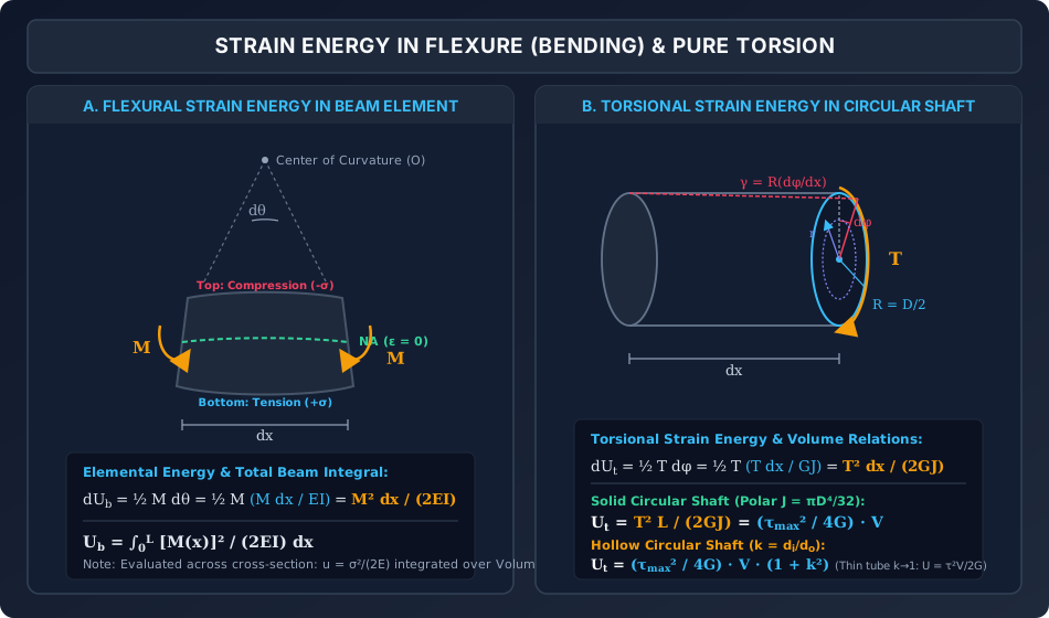
  10. Diagram 1: Bending & Torsional Strain Energy Mechanisms
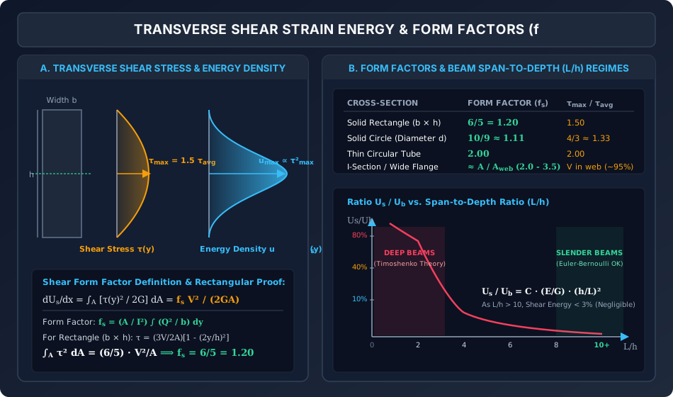
  11. Diagram 2: Transverse Shear Stress, Energy Density & Form Factors
  12. 4. Comprehensive Comparison Tables
  13. Table 1: Governing Strain Energy Expressions for Primary Loading Modes
  14. Table 2: Shear Form Factors (fs) and Stress Ratios for Structural Cross Sections
  15. 5. Fully Solved Numerical Examples
  16. Example 1: Cantilever Beam under Combined Point Load and UDL (Coupling & Deflection)
  17. Example 2: Elastic Energy Storage Capacity of Solid vs. Hollow Shafts
  18. Example 3: Deep Rectangular Timber Beam — Exact Shear vs. Bending Energy Partition
  19. 6. Common Misconceptions & High-Yield Exam Traps
  20. Misconception 1: "Superposition of strain energy is valid because forces superpose"
  21. Misconception 2: "Torsional strain energy in a solid shaft is fracτmax22G V"
  22. Misconception 3: "The shear form factor fs equals the ratio τmax / τavg"
  23. Misconception 4: "Castigliano's theorem can only find deflections where real loads exist"
  24. Misconception 5: "Euler-Bernoulli beam theory is always acceptable for bridge girders"
  25. 7. Previous Years Questions & Benchmark Solutions
  26. Question 1 (GATE CE)
  27. Question 2 (UPSC ESE)
  28. Question 3 (SSC JE / State AE)
  29. 8. Indian Standard (IS) Code References & Design Implications
  30. 9. Quick Revision Formulas & Key Exam Takeaways

Metadata

  • Topic ID: SOM-10-02
  • Module: Subject 02: Strength of Materials
  • Chapter: Chapter 10: Strain Energy & Impact Loading
  • Author: Civil Engineering Autonomous Content & QA Agent
  • Standard Reference: IS 456:2000, IS 800:2007, IS 883:1994, IRC:21-2000
  • Target Examinations: GATE CE, UPSC ESE, SSC JE, State AE/JE, RRB JE

1. Engineering Fundamentals & Theoretical Basis

In structural mechanics, when an elastic member deforms under external loads, work is transferred from the external applied forces into internal strain energy stored throughout the continuum. For a linearly elastic, homogeneous, isotropic material obeying Hooke's Law, the general three-dimensional elastic strain energy stored in an elastic body of volume VV is given by:

U=12∫V(σxϵx+σyϵy+σzϵz+τxyγxy+τyzγyz+τzxγzx)dVU = \frac{1}{2} \int_V \left( \sigma_x \epsilon_x + \sigma_y \epsilon_y + \sigma_z \epsilon_z + \tau_{xy} \gamma_{xy} + \tau_{yz} \gamma_{yz} + \tau_{zx} \gamma_{zx} \right) dV

Expressing strains in terms of stresses using Hooke's Law:

u=12E(σx2+σy2+σz2−2ν(σxσy+σyσz+σzσx))+12G(τxy2+τyz2+τzx2)u = \frac{1}{2E} \left( \sigma_x^2 + \sigma_y^2 + \sigma_z^2 - 2\nu(\sigma_x \sigma_y + \sigma_y \sigma_z + \sigma_z \sigma_x) \right) + \frac{1}{2G} \left( \tau_{xy}^2 + \tau_{yz}^2 + \tau_{zx}^2 \right)

When dealing with slender structural elements such as beams, columns, and shafts, this general continuum expression simplifies into three fundamental structural loading modes:

  1. Flexural Strain Energy (UbU_b): Internal work stored due to normal bending stresses σ(y)=MyI\sigma(y) = \frac{M y}{I} resisting applied bending moments M(x)M(x).
  2. Torsional Strain Energy (UtU_t): Internal work stored due to shear stresses τ(r)=TrJ\tau(r) = \frac{T r}{J} resisting applied twisting moments T(x)T(x).
  3. Transverse Shear Strain Energy (UsU_s): Internal work stored due to transverse shear stresses τ(y)=VQIb\tau(y) = \frac{V Q}{I b} resisting beam shear forces V(x)V(x).

Work-Energy Equilibrium & Castigliano's Theorems

By the Principle of Conservation of Energy, for a system gradually loaded from rest in static equilibrium without thermal dissipation:

Wext=Uinternal=Ua+Ub+Ut+UsW_{\text{ext}} = U_{\text{internal}} = U_a + U_b + U_t + U_s

For linearly elastic structures where strain energy UU is equal to complementary strain energy U∗U^*:

  • Castigliano's First Theorem: The partial derivative of total strain energy with respect to a displacement component Δi\Delta_i yields the corresponding generalized force PiP_i: ∂U∂Δi=Pi\frac{\partial U}{\partial \Delta_i} = P_i
  • Castigliano's Second Theorem: The partial derivative of total strain energy with respect to an applied generalized force PiP_i yields the deflection (or rotation) Δi\Delta_i along the line of action of that force: ∂U∂Pi=Δi,∂U∂Mi=θi\frac{\partial U}{\partial P_i} = \Delta_i, \quad \frac{\partial U}{\partial M_i} = \theta_i

2. Mathematical Derivations & Complete Proofs

2.1 Derivation 1: Strain Energy in Pure Flexure (Bending)

Consider an infinitesimal beam segment of length dxdx, flexural rigidity EI(x)EI(x), subjected to a bending moment M(x)M(x).

   M(x)  ┌──────────────────┐  M(x) + dM
  -----> │                  │ ----->
         │                  │
  <----- │        dx        │ <-----
         └──────────────────┘

Method A: Direct Work Done by Elemental Curvature

The relative angular rotation dθd\theta of the two facing cross-sections over the span dxdx is given by the differential equation of beam flexure:

dθ=κ dx=M(x)EI dxd\theta = \kappa \, dx = \frac{M(x)}{EI} \, dx

Since the bending moment increases linearly from 00 to M(x)M(x) during gradual elastic application, the incremental external work done (and thus the internal flexural strain energy dUbdU_b stored) is:

dUb=12M(x) dθ=12M(x)(M(x)EI dx)=[M(x)]22EI dxdU_b = \frac{1}{2} M(x) \, d\theta = \frac{1}{2} M(x) \left( \frac{M(x)}{EI} \, dx \right) = \frac{[M(x)]^2}{2EI} \, dx

Integrating over the entire beam length LL:

Ub=∫0L[M(x)]22EI dxU_b = \int_0^L \frac{[M(x)]^2}{2EI} \, dx

Method B: Continuum Volume Integration of Normal Stress

Using the Navier flexure formula, the longitudinal normal stress at distance yy from the neutral axis is:

σ(x,y)=M(x) yI\sigma(x, y) = \frac{M(x) \, y}{I}

The strain energy density at that point is:

u(x,y)=σ(x,y)22E=[M(x)]2y22EI2u(x, y) = \frac{\sigma(x, y)^2}{2E} = \frac{[M(x)]^2 y^2}{2E I^2}

Integrating over the differential volume dV=dA⋅dxdV = dA \cdot dx:

dUb=[∫A[M(x)]2y22EI2 dA]dx=[M(x)]22EI2[∫Ay2 dA]dxdU_b = \left[ \int_A \frac{[M(x)]^2 y^2}{2E I^2} \, dA \right] dx = \frac{[M(x)]^2}{2E I^2} \left[ \int_A y^2 \, dA \right] dx

By definition of the second moment of area, ∫Ay2dA=I\int_A y^2 dA = I. Substituting:

dUb=[M(x)]22EI2⋅I dx=[M(x)]22EI dx  ⟹  Ub=∫0L[M(x)]22EI dxdU_b = \frac{[M(x)]^2}{2E I^2} \cdot I \, dx = \frac{[M(x)]^2}{2EI} \, dx \implies U_b = \int_0^L \frac{[M(x)]^2}{2EI} \, dx

Both methods yield identical results, confirming theoretical rigor.


2.2 Derivation 2: Strain Energy in Pure Torsion of Circular Shafts

Consider an infinitesimal shaft segment of length dxdx, torsional rigidity GJGJ, subjected to twisting moment T(x)T(x).

Method A: Work Done by Torsional Rotation

The relative angle of twist dϕd\phi over length dxdx is:

dϕ=T(x)GJ dxd\phi = \frac{T(x)}{GJ} \, dx

The incremental torsional strain energy is:

dUt=12T(x) dϕ=12T(x)(T(x)GJ dx)=[T(x)]22GJ dxdU_t = \frac{1}{2} T(x) \, d\phi = \frac{1}{2} T(x) \left( \frac{T(x)}{GJ} \, dx \right) = \frac{[T(x)]^2}{2GJ} \, dx

Integrating along the length:

Ut=∫0L[T(x)]22GJ dxU_t = \int_0^L \frac{[T(x)]^2}{2GJ} \, dx

For a uniform prismatic shaft of length LL under constant torque TT:

Ut=T2L2GJU_t = \frac{T^2 L}{2GJ}

Method B: Expressed in Terms of Maximum Surface Shear Stress τmax⁡\tau_{\max}

From the torsion formula:

TJ=τ(r)r=τmax⁡R  ⟹  T=τmax⁡JR\frac{T}{J} = \frac{\tau(r)}{r} = \frac{\tau_{\max}}{R} \implies T = \frac{\tau_{\max} J}{R}

Substitute TT into the strain energy formula:

Ut=(τmax⁡JR)2L2GJ=τmax⁡2JL2GR2U_t = \frac{\left( \frac{\tau_{\max} J}{R} \right)^2 L}{2GJ} = \frac{\tau_{\max}^2 J L}{2 G R^2}
Case 1: Solid Circular Shaft (D=2RD = 2R)
  • Polar moment of inertia: J=πD432=πR42J = \frac{\pi D^4}{32} = \frac{\pi R^4}{2}
  • Volume of shaft: V=πD24L=πR2LV = \frac{\pi D^2}{4} L = \pi R^2 L

Substituting JJ:

Ut=τmax⁡2(πR42)L2GR2=τmax⁡2(πR2L)4G=τmax⁡24GVU_t = \frac{\tau_{\max}^2 \left( \frac{\pi R^4}{2} \right) L}{2 G R^2} = \frac{\tau_{\max}^2 (\pi R^2 L)}{4G} = \frac{\tau_{\max}^2}{4G} V

Crucial Exam Result: The total torsional strain energy stored in a solid circular shaft is exactly half of the product of pure shear energy density at the outer fiber (τmax⁡22G\frac{\tau_{\max}^2}{2G}) and the total volume VV, because shear stress drops linearly to zero at the shaft centerline.

Case 2: Hollow Circular Shaft (Do=2RoD_o = 2R_o, Di=2RiD_i = 2R_i, diameter ratio k=Di/Dok = D_i / D_o)
  • Polar moment: J=π(Do4−Di4)32=πDo4(1−k4)32=πRo4(1−k4)2J = \frac{\pi (D_o^4 - D_i^4)}{32} = \frac{\pi D_o^4 (1 - k^4)}{32} = \frac{\pi R_o^4 (1 - k^4)}{2}
  • Volume: V=π(Do2−Di2)4L=πDo2(1−k2)4L=πRo2(1−k2)LV = \frac{\pi (D_o^2 - D_i^2)}{4} L = \frac{\pi D_o^2 (1 - k^2)}{4} L = \pi R_o^2 (1 - k^2) L

Substitute into UtU_t:

Ut=τmax⁡2[πRo4(1−k4)2]L2GRo2=τmax⁡2πRo2L(1−k4)4G=τmax⁡2[πRo2L(1−k2)](1+k2)4GU_t = \frac{\tau_{\max}^2 \left[ \frac{\pi R_o^4 (1 - k^4)}{2} \right] L}{2 G R_o^2} = \frac{\tau_{\max}^2 \pi R_o^2 L (1 - k^4)}{4G} = \frac{\tau_{\max}^2 \left[ \pi R_o^2 L (1 - k^2) \right] (1 + k^2)}{4G} Ut=τmax⁡24GV⋅(1+k2)U_t = \frac{\tau_{\max}^2}{4G} V \cdot (1 + k^2)

When k→0k \to 0 (solid shaft), Ut=τmax⁡24GVU_t = \frac{\tau_{\max}^2}{4G} V.
When k→1k \to 1 (very thin-walled tube), (1+k2)→2(1 + k^2) \to 2, giving:

Ut,thin tube=τmax⁡22GVU_{t,\text{thin tube}} = \frac{\tau_{\max}^2}{2G} V

This matches pure uniform shear energy density, because in a thin tube all material is concentrated at maximum radius RoR_o.


2.3 Derivation 3: Transverse Shear Strain Energy & Form Factors (fsf_s)

In a beam subjected to transverse shear force V(x)V(x), the shear stress across the depth is non-uniform and given by Jourawski's shear formula:

τ(y)=V(x)Q(y)I b(y)\tau(y) = \frac{V(x) Q(y)}{I \, b(y)}

The shear strain energy stored in an elemental volume dV=b(y)dy dxdV = b(y) dy \, dx is:

dUs=∫Aτ(y)22G dA dx=(V22GI2∫AQ(y)2b(y) dy)dxdU_s = \int_A \frac{\tau(y)^2}{2G} \, dA \, dx = \left( \frac{V^2}{2G I^2} \int_A \frac{Q(y)^2}{b(y)} \, dy \right) dx

To express this in the standard engineering form:

dUs=fs[V(x)]22GA dx  ⟹  Us=∫0Lfs[V(x)]22GA dxdU_s = \frac{f_s [V(x)]^2}{2GA} \, dx \implies U_s = \int_0^L \frac{f_s [V(x)]^2}{2GA} \, dx

Equating the two expressions defines the Shear Form Factor (also called the shape factor for shear deformation or Timoshenko shear coefficient κ=1/fs\kappa = 1/f_s):

fs=AI2∫A[Q(y)]2b(y)2 dA=AI2∫−h/2h/2[Q(y)]2b(y) dyf_s = \frac{A}{I^2} \int_A \frac{[Q(y)]^2}{b(y)^2} \, dA = \frac{A}{I^2} \int_{-h/2}^{h/2} \frac{[Q(y)]^2}{b(y)} \, dy

Derivation for Solid Rectangular Cross-Section (b×hb \times h)

  • Area: A=bhA = bh
  • Second moment: I=bh312I = \frac{bh^3}{12}
  • First moment of area of fiber above yy: Q(y)=∫yh/2η b dη=b2(h24−y2)Q(y) = \int_y^{h/2} \eta \, b \, d\eta = \frac{b}{2} \left( \frac{h^2}{4} - y^2 \right)
  • Shear stress distribution: τ(y)=V⋅b2(h24−y2)(bh312)b=6Vbh3(h24−y2)=3V2A[1−(2yh)2]\tau(y) = \frac{V \cdot \frac{b}{2} \left( \frac{h^2}{4} - y^2 \right)}{\left(\frac{bh^3}{12}\right) b} = \frac{6V}{bh^3} \left( \frac{h^2}{4} - y^2 \right) = \frac{3V}{2A} \left[ 1 - \left(\frac{2y}{h}\right)^2 \right]

Now integrate τ(y)2\tau(y)^2 across the cross section:

∫Aτ(y)2dA=b∫−h/2h/2(3V2A)2[1−8y2h2+16y4h4]dy\int_A \tau(y)^2 dA = b \int_{-h/2}^{h/2} \left( \frac{3V}{2A} \right)^2 \left[ 1 - \frac{8y^2}{h^2} + \frac{16y^4}{h^4} \right] dy =b(9V24A2)[y−8y33h2+16y55h4]−h/2h/2=b(9V24A2)2[h2−8(h/2)33h2+16(h/2)55h4]= b \left(\frac{9V^2}{4A^2}\right) \left[ y - \frac{8y^3}{3h^2} + \frac{16y^5}{5h^4} \right]_{-h/2}^{h/2} = b \left(\frac{9V^2}{4A^2}\right) 2 \left[ \frac{h}{2} - \frac{8(h/2)^3}{3h^2} + \frac{16(h/2)^5}{5h^4} \right] =b(9V24A2)h[1−23+15]=(bh)(9V24A2)[815]=7260V2A=65V2A= b \left(\frac{9V^2}{4A^2}\right) h \left[ 1 - \frac{2}{3} + \frac{1}{5} \right] = (bh) \left(\frac{9V^2}{4A^2}\right) \left[ \frac{8}{15} \right] = \frac{72}{60} \frac{V^2}{A} = \frac{6}{5} \frac{V^2}{A}

Equating to fsV2A\frac{f_s V^2}{A}:

fs=65=1.20f_s = \frac{6}{5} = 1.20

Summary of Shear Form Factors for Standard Civil Engineering Sections:

  1. Solid Rectangle: fs=65=1.20f_s = \frac{6}{5} = 1.20
  2. Solid Circle: fs=109≈1.111f_s = \frac{10}{9} \approx 1.111
  3. Thin-Walled Circular Tube: fs=2.00f_s = 2.00
  4. Diamond / Rhombus: fs=65=1.20f_s = \frac{6}{5} = 1.20
  5. I-Section / Flanged Girder: fs≈AtotalAweb≈2.0 to 3.5f_s \approx \frac{A_{\text{total}}}{A_{\text{web}}} \approx 2.0 \text{ to } 3.5 (since the web carries ≈90–95%\approx 90\text{--}95\% of total shear force).

2.4 Derivation 4: Ratio of Shear to Flexural Strain Energy & Timoshenko Threshold

To evaluate when transverse shear strain energy can be safely neglected in structural analysis, consider a simply supported beam of rectangular section (b×hb \times h), length LL, carrying a central point load PP.

         P
         ↓
  ▲═════════════▲
  x=0    L/2    L

1. Flexural Strain Energy (UbU_b):

For 0≤x≤L/20 \le x \le L/2, M(x)=Px2M(x) = \frac{P x}{2}:

Ub=2∫0L/2(Px/2)22EI dx=P24EI[x33]0L/2=P2L396EIU_b = 2 \int_0^{L/2} \frac{(Px/2)^2}{2EI} \, dx = \frac{P^2}{4EI} \left[ \frac{x^3}{3} \right]_0^{L/2} = \frac{P^2 L^3}{96 EI}

2. Transverse Shear Strain Energy (UsU_s):

For the entire beam, ∣V(x)∣=P2|V(x)| = \frac{P}{2}:

Us=∫0Lfs[V(x)]22GA dx=fs(P/2)2L2GA=fsP2L8GAU_s = \int_0^L \frac{f_s [V(x)]^2}{2GA} \, dx = \frac{f_s (P/2)^2 L}{2GA} = \frac{f_s P^2 L}{8GA}

3. Energy Ratio:

Dividing UsU_s by UbU_b:

UsUb=fsP2L8GAP2L396EI=12fs EIGA L2\frac{U_s}{U_b} = \frac{\frac{f_s P^2 L}{8GA}}{\frac{P^2 L^3}{96 EI}} = \frac{12 f_s \, EI}{GA \, L^2}

For a rectangular cross-section, fs=1.2f_s = 1.2, I=bh312I = \frac{bh^3}{12}, A=bh  ⟹  IA=h212A = bh \implies \frac{I}{A} = \frac{h^2}{12}:

UsUb=12(1.2) E(h212)G L2=1.2(EG)(hL)2\frac{U_s}{U_b} = \frac{12 (1.2) \, E \left(\frac{h^2}{12}\right)}{G \, L^2} = 1.2 \left( \frac{E}{G} \right) \left( \frac{h}{L} \right)^2

Relating elastic moduli via G=E2(1+ν)G = \frac{E}{2(1 + \nu)}:

UsUb=2.4(1+ν)(hL)2\frac{U_s}{U_b} = 2.4 (1 + \nu) \left( \frac{h}{L} \right)^2

For structural steel (ν=0.30\nu = 0.30):

UsUb≈3.12(hL)2\frac{U_s}{U_b} \approx 3.12 \left( \frac{h}{L} \right)^2
Physical Engineering Implications:
  • Slender Beams (L/h≥10L/h \ge 10): UsUb≤3.12(110)2=0.0312  ⟹  3.12%\frac{U_s}{U_b} \le 3.12 \left( \frac{1}{10} \right)^2 = 0.0312 \implies \mathbf{3.12\%} Shear strain energy accounts for under 3.2%3.2\% of total deformation energy. Euler-Bernoulli beam theory (which assumes plane sections remain plane and normal to the neutral axis, ignoring shear strain) is valid with <3%<3\% error.
  • Deep Beams (L/h≤4L/h \le 4): UsUb≥3.12(14)2=0.195  ⟹  19.5% to 75%+\frac{U_s}{U_b} \ge 3.12 \left( \frac{1}{4} \right)^2 = 0.195 \implies \mathbf{19.5\% \text{ to } 75\%+} Shear strain energy and shear deformations become dominant. Timoshenko beam theory or two-dimensional elasticity (strut-and-tie models per IS 456 Annexure) must be applied.

3. Engineering Visualizations & Technical Diagrams

Diagram 1: Bending & Torsional Strain Energy Mechanisms

The schematic below visualizes the internal curvature and angular twist governing strain energy in flexural beam segments and cylindrical shafts.

Strain Energy in Bending and Pure Torsion

Analytical Walk-Through:

  1. Flexural Deformation (Panel A): Shows an infinitesimal element dxdx bending through angle dθ=MEIdxd\theta = \frac{M}{EI} dx. The triangular normal stress distribution stores strain energy u=σ22Eu = \frac{\sigma^2}{2E} symmetrically about the neutral axis, integrating to Ub=∫M22EIdxU_b = \int \frac{M^2}{2EI} dx.
  2. Torsional Deformation (Panel B): Shows an elemental shaft segment dxdx twisting through angle dϕ=TGJdxd\phi = \frac{T}{GJ} dx. The shear stress increases linearly with radius rr, producing an internal energy integral of τmax⁡24GV\frac{\tau_{\max}^2}{4G} V for solid shafts, and τmax⁡24GV(1+k2)\frac{\tau_{\max}^2}{4G} V (1+k^2) for hollow shafts.

Diagram 2: Transverse Shear Stress, Energy Density & Form Factors

The figure below depicts the parabolic distribution of shear stress, the quartic energy density profile, and the relationship between span-to-depth ratio (L/hL/h) and shear-to-bending energy ratios.

Transverse Shear Strain Energy and Form Factors

Analytical Walk-Through:

  1. Stress vs. Energy Profiles (Panel A): While shear stress τ(y)\tau(y) is parabolic, strain energy density us(y)=τ22Gu_s(y) = \frac{\tau^2}{2G} is a quartic curve sharply peaked at the neutral axis. This non-linear concentration creates the form factor fs=6/5=1.20f_s = 6/5 = 1.20.
  2. Span-to-Depth Ratio Regimes (Panel B & C): Demonstrates that as L/hL/h drops below 55, the shear energy curve climbs rapidly as (h/L)2(h/L)^2, demarcating the transition from Euler-Bernoulli slender beam behavior to Timoshenko deep beam behavior.

4. Comprehensive Comparison Tables

Table 1: Governing Strain Energy Expressions for Primary Loading Modes

Loading Mode Internal Force / Moment Kinematic Deformation Strain Energy Increment (dUdU) Total Strain Energy (UU) Energy in Terms of Peak Stress
Axial (Tension/Comp.) Axial Force P(x)P(x) Elongation dΔ=PAEdxd\Delta = \frac{P}{AE} dx P22AEdx\frac{P^2}{2AE} dx ∫0LP22AEdx\int_0^L \frac{P^2}{2AE} dx σmax⁡22EV\frac{\sigma_{\max}^2}{2E} V (uniform)
Pure Flexure (Bending) Bending Moment M(x)M(x) Curvature dθ=MEIdxd\theta = \frac{M}{EI} dx M22EIdx\frac{M^2}{2EI} dx ∫0LM22EIdx\int_0^L \frac{M^2}{2EI} dx σmax⁡26EV\frac{\sigma_{\max}^2}{6E} V (rectangle)
Pure Torsion (Circular) Twisting Moment T(x)T(x) Angle of Twist dϕ=TGJdxd\phi = \frac{T}{GJ} dx T22GJdx\frac{T^2}{2GJ} dx ∫0LT22GJdx\int_0^L \frac{T^2}{2GJ} dx τmax⁡24GV\frac{\tau_{\max}^2}{4G} V (solid)
Transverse Shear Shear Force V(x)V(x) Shear Distortion dγd\gamma fsV22GAdx\frac{f_s V^2}{2GA} dx ∫0LfsV22GAdx\int_0^L \frac{f_s V^2}{2GA} dx fs⋅τavg22GVf_s \cdot \frac{\tau_{\text{avg}}^2}{2G} V

Table 2: Shear Form Factors (fsf_s) and Stress Ratios for Structural Cross Sections

Cross-Sectional Geometry Shear Form Factor (fsf_s) Peak Shear Stress (τmax⁡\tau_{\max}) Effective Shear Area (As=A/fsA_s = A / f_s) Practical Usage
Solid Rectangle (b×hb \times h) 65=1.20\frac{6}{5} = 1.20 1.50 τavg1.50 \, \tau_{\text{avg}} 56A≈0.833A\frac{5}{6} A \approx 0.833 A Timber beams, RC rectangular beams
Solid Circle (Diameter DD) 109≈1.111\frac{10}{9} \approx 1.111 43τavg≈1.333τavg\frac{4}{3} \tau_{\text{avg}} \approx 1.333 \tau_{\text{avg}} 0.90A0.90 A Circular columns, bridge piers
Thin Circular Tube (t≪Dt \ll D) 2.002.00 2.00 τavg2.00 \, \tau_{\text{avg}} 0.50A0.50 A Tubular structural steel trusses
Diamond / Rhombus 65=1.20\frac{6}{5} = 1.20 98τavg=1.125τavg\frac{9}{8} \tau_{\text{avg}} = 1.125 \tau_{\text{avg}} 0.833A0.833 A Architectural sections
I-Girder / Wide Flange ≈AtotalAweb≈2.0–3.5\approx \frac{A_{\text{total}}}{A_{\text{web}}} \approx 2.0\text{--}3.5 ≈VAweb\approx \frac{V}{A_{\text{web}}} ≈Aweb\approx A_{\text{web}} Rolled steel beams (ISMB, ISWB)

5. Fully Solved Numerical Examples

Example 1: Cantilever Beam under Combined Point Load and UDL (Coupling & Deflection)

Problem Statement:
A prismatic structural steel cantilever beam of length L=3.0 mL = 3.0\text{ m} is rigidly clamped at x=Lx = L and free at x=0x = 0. It carries a concentrated downward vertical load P=15 kNP = 15\text{ kN} at the free tip and a uniformly distributed downward load w=10 kN/mw = 10\text{ kN/m} across its entire length.
Given: E=200 GPaE = 200\text{ GPa}, second moment of area I=8.0×10⁻⁵ m4I = 8.0 \times 10^{-5}\text{ m}^4.

  1. Calculate the total flexural strain energy UbU_b stored in the beam.
  2. Determine the proportion of strain energy attributable to the coupling (mutual work) between PP and ww.
  3. Using Castigliano's Theorem, compute the total vertical deflection δtip\delta_{\text{tip}} at the free tip.

Step 1: Establish the Bending Moment Function M(x)M(x)

Take coordinate xx measured from the free end (x=0x = 0) towards the fixed base (x=Lx = L):

M(x)=Px+wx22M(x) = P x + \frac{w x^2}{2}

Compute the square of the bending moment:

[M(x)]2=(Px+wx22)2=P2x2+Pwx3+w2x44[M(x)]^2 = \left( P x + \frac{w x^2}{2} \right)^2 = P^2 x^2 + P w x^3 + \frac{w^2 x^4}{4}

Step 2: Integrate to Find Total Strain Energy UbU_b

Ub=12EI∫0L[M(x)]2 dx=12EI[P2∫0Lx2dx+Pw∫0Lx3dx+w24∫0Lx4dx]U_b = \frac{1}{2EI} \int_0^L [M(x)]^2 \, dx = \frac{1}{2EI} \left[ P^2 \int_0^L x^2 dx + P w \int_0^L x^3 dx + \frac{w^2}{4} \int_0^L x^4 dx \right] Ub=12EI[P2L33+PwL44+w2L520]U_b = \frac{1}{2EI} \left[ \frac{P^2 L^3}{3} + \frac{P w L^4}{4} + \frac{w^2 L^5}{20} \right]

Substitute numerical quantities:

  • EI=200×109×8.0×10−5=1.60×10⁷ N⋅m2=16.0 MN⋅m2EI = 200 \times 10^9 \times 8.0 \times 10^{-5} = 1.60 \times 10^7\text{ N}\cdot\text{m}^2 = 16.0\text{ MN}\cdot\text{m}^2
  • P=15 000 NP = 15\,000\text{ N}
  • w=10 000 N/mw = 10\,000\text{ N/m}
  • L=3.0 mL = 3.0\text{ m}

Evaluate the individual bracket terms:

  • Term 1 (Load PP acting alone): Term1=P2L33=(15 000)2×(3)33=2.25×108×273=2.025×10⁹ N2⋅m3\text{Term}_1 = \frac{P^2 L^3}{3} = \frac{(15\,000)^2 \times (3)^3}{3} = \frac{2.25 \times 10^8 \times 27}{3} = 2.025 \times 10^9\text{ N}^2\cdot\text{m}^3
  • Term 2 (Mutual coupling work): Term2=PwL44=15 000×10 000×(3)44=1.5×108×814=3.0375×10⁹ N2⋅m3\text{Term}_2 = \frac{P w L^4}{4} = \frac{15\,000 \times 10\,000 \times (3)^4}{4} = \frac{1.5 \times 10^8 \times 81}{4} = 3.0375 \times 10^9\text{ N}^2\cdot\text{m}^3
  • Term 3 (UDL ww acting alone): Term3=w2L520=(10 000)2×(3)520=1.0×108×24320=1.215×10⁹ N2⋅m3\text{Term}_3 = \frac{w^2 L^5}{20} = \frac{(10\,000)^2 \times (3)^5}{20} = \frac{1.0 \times 10^8 \times 243}{20} = 1.215 \times 10^9\text{ N}^2\cdot\text{m}^3

Sum of bracketed terms:

Σ=2.025×10⁹+3.0375×10⁹+1.215×109=6.2775×10⁹ N2⋅m3\Sigma = 2.025 \times 10^9 + 3.0375 \times 10^9 + 1.215 \times 10^9 = 6.2775 \times 10^9\text{ N}^2\cdot\text{m}^3

Total flexural strain energy:

Ub=6.2775×1092×(1.60×107)=6.2775×1093.20×107=196.1719 JoulesU_b = \frac{6.2775 \times 10^9}{2 \times (1.60 \times 10^7)} = \frac{6.2775 \times 10^9}{3.20 \times 10^7} = \mathbf{196.1719\text{ Joules}}

Step 3: Energy Decomposition & Coupling Analysis

  • Strain energy from PP alone: UP=2.025×1093.20×107=63.2813 JU_P = \frac{2.025 \times 10^9}{3.20 \times 10^7} = 63.2813\text{ J} (32.26%32.26\%)
  • Strain energy from ww alone: Uw=1.215×1093.20×107=37.9688 JU_w = \frac{1.215 \times 10^9}{3.20 \times 10^7} = 37.9688\text{ J} (19.35%19.35\%)
  • Coupling / interaction energy: UPw=3.0375×1093.20×107=94.9219 JU_{Pw} = \frac{3.0375 \times 10^9}{3.20 \times 10^7} = \mathbf{94.9219\text{ J}} (48.39%48.39\%)

Critical Insight: The mutual coupling term accounts for nearly half (48.4%48.4\%) of the total stored strain energy. Strain energy is a quadratic function; superposition of strain energy (Utotal=U1+U2U_{\text{total}} = U_1 + U_2) is mathematically invalid whenever loads act simultaneously!

Step 4: Vertical Tip Deflection via Castigliano's Theorem

Apply Castigliano's Second Theorem:

δtip=∂Ub∂P=1EI∫0LM(x)∂M∂P dx\delta_{\text{tip}} = \frac{\partial U_b}{\partial P} = \frac{1}{EI} \int_0^L M(x) \frac{\partial M}{\partial P} \, dx

Since ∂M(x)∂P=x\frac{\partial M(x)}{\partial P} = x:

δtip=1EI∫0L(Px+wx22)x dx=1EI[PL33+wL48]\delta_{\text{tip}} = \frac{1}{EI} \int_0^L \left( P x + \frac{w x^2}{2} \right) x \, dx = \frac{1}{EI} \left[ \frac{P L^3}{3} + \frac{w L^4}{8} \right]

Substitute the values:

  • From PP: PL33EI=15 000×273×1.60×107=405 0004.80×107=0.0084375 m=8.4375 mm\frac{P L^3}{3 EI} = \frac{15\,000 \times 27}{3 \times 1.60 \times 10^7} = \frac{405\,000}{4.80 \times 10^7} = 0.0084375\text{ m} = 8.4375\text{ mm}
  • From ww: wL48EI=10 000×818×1.60×107=810 0001.28×108=0.0063281 m=6.3281 mm\frac{w L^4}{8 EI} = \frac{10\,000 \times 81}{8 \times 1.60 \times 10^7} = \frac{810\,000}{1.28 \times 10^8} = 0.0063281\text{ m} = 6.3281\text{ mm}

Total tip deflection:

δtip=8.4375+6.3281=14.7656 mm\delta_{\text{tip}} = 8.4375 + 6.3281 = \mathbf{14.7656\text{ mm}}

Example 2: Elastic Energy Storage Capacity of Solid vs. Hollow Shafts

Problem Statement:
An alloy steel drive shaft of length L=2.0 mL = 2.0\text{ m} is designed to operate under pure torsion with a shear modulus G=80 GPaG = 80\text{ GPa} and an allowable maximum shear stress τallow=60 MPa\tau_{\text{allow}} = 60\text{ MPa}.
Compare two alternative designs having identical total material volume (and mass):

  • Design A: Solid circular shaft of diameter DsD_s.
  • Design B: Hollow circular shaft with outer diameter Do=100 mmD_o = 100\text{ mm} and inner diameter Di=60 mmD_i = 60\text{ mm} (k=Di/Do=0.60k = D_i / D_o = 0.60).

Calculate:

  1. The required solid shaft diameter DsD_s.
  2. The total torsional strain energy stored in both shafts at their allowable limit.
  3. The torque transmission capacity ratio Thollow/TsolidT_{\text{hollow}} / T_{\text{solid}}.

Step 1: Find Solid Diameter DsD_s for Equal Mass

Equal mass requires equal cross-sectional area:

As=Ah  ⟹  π4Ds2=π4(Do2−Di2)=π4Do2(1−k2)A_s = A_h \implies \frac{\pi}{4} D_s^2 = \frac{\pi}{4} (D_o^2 - D_i^2) = \frac{\pi}{4} D_o^2 (1 - k^2) Ds=Do1−k2=1001−0.62=1000.64=80.0 mmD_s = D_o \sqrt{1 - k^2} = 100 \sqrt{1 - 0.6^2} = 100 \sqrt{0.64} = \mathbf{80.0\text{ mm}}

Total volume of both shafts:

V=A⋅L=(π4×0.0802)×2.0=5.0265×10−3×2.0=0.010053 m3V = A \cdot L = \left( \frac{\pi}{4} \times 0.080^2 \right) \times 2.0 = 5.0265 \times 10^{-3} \times 2.0 = \mathbf{0.010053\text{ m}^3}

Step 2: Torsional Strain Energy Stored

  • Solid Shaft:

    Usolid=τmax⁡24GV=(60×106)24×(80×109)×0.010053=3.60×10153.20×1011×0.010053=11 250×0.010053=113.0973 JoulesU_{\text{solid}} = \frac{\tau_{\max}^2}{4G} V = \frac{(60 \times 10^6)^2}{4 \times (80 \times 10^9)} \times 0.010053 = \frac{3.60 \times 10^{15}}{3.20 \times 10^{11}} \times 0.010053 = 11\,250 \times 0.010053 = \mathbf{113.0973\text{ Joules}}
  • Hollow Shaft (k=0.6k = 0.6):

    Uhollow=τmax⁡24GV(1+k2)=Usolid(1+0.62)=113.0973×(1+0.36)=153.8124 JoulesU_{\text{hollow}} = \frac{\tau_{\max}^2}{4G} V (1 + k^2) = U_{\text{solid}} (1 + 0.6^2) = 113.0973 \times (1 + 0.36) = \mathbf{153.8124\text{ Joules}}

Energy Storage Ratio:

UhollowUsolid=1+k2=1.3600  ⟹  +36.0% greater energy capacity!\frac{U_{\text{hollow}}}{U_{\text{solid}}} = 1 + k^2 = 1.3600 \implies \mathbf{+36.0\% \text{ greater energy capacity!}}

Step 3: Torque Transmission Capacity

  • Solid shaft torque capacity: Tsolid=π16τmax⁡Ds3=π16×(60×106)×(0.080)3=6 031.86 N⋅mT_{\text{solid}} = \frac{\pi}{16} \tau_{\max} D_s^3 = \frac{\pi}{16} \times (60 \times 10^6) \times (0.080)^3 = \mathbf{6\,031.86\text{ N}\cdot\text{m}}
  • Hollow shaft torque capacity: Thollow=π16τmax⁡Do3(1−k4)=π16×(60×106)×(0.100)3×(1−0.64)T_{\text{hollow}} = \frac{\pi}{16} \tau_{\max} D_o^3 (1 - k^4) = \frac{\pi}{16} \times (60 \times 10^6) \times (0.100)^3 \times (1 - 0.6^4) =11 780.97×(1−0.1296)=11 780.97×0.8704=10 254.16 N⋅m= 11\,780.97 \times (1 - 0.1296) = 11\,780.97 \times 0.8704 = \mathbf{10\,254.16\text{ N}\cdot\text{m}}

Torque Capacity Ratio:

ThollowTsolid=10 254.166 031.86=1.7000  ⟹  +70.0% greater torque!\frac{T_{\text{hollow}}}{T_{\text{solid}}} = \frac{10\,254.16}{6\,031.86} = \mathbf{1.7000 \implies +70.0\% \text{ greater torque!}}

Takeaway: For the exact same mass of material, a hollow shaft (k=0.6k=0.6) carries 70%70\% more torque and absorbs 36%36\% more torsional impact strain energy before yielding.


Example 3: Deep Rectangular Timber Beam — Exact Shear vs. Bending Energy Partition

Problem Statement:
A short, deep timber beam of rectangular cross-section (b=150 mmb = 150\text{ mm}, h=300 mmh = 300\text{ mm}) spans simply supported over length L=1.20 mL = 1.20\text{ m}. It is subjected to a central concentrated vertical load P=40 kNP = 40\text{ kN}.
Timber properties: E=12.0 GPaE = 12.0\text{ GPa}, shear modulus G=1.20 GPaG = 1.20\text{ GPa} (E/G=10E/G = 10).
Calculate:

  1. The flexural strain energy UbU_b.
  2. The transverse shear strain energy UsU_s.
  3. The percentage ratio Us/UbU_s / U_b.
  4. The flexural deflection δb\delta_b, shear deflection δs\delta_s, and the total central deflection δtotal\delta_{\text{total}}.

Step 1: Geometric & Material Properties

  • Span-to-depth ratio: Lh=1.200.30=4.0\frac{L}{h} = \frac{1.20}{0.30} = 4.0 (Deep beam regime)
  • Area: A=0.150×0.300=0.0450 m2A = 0.150 \times 0.300 = 0.0450\text{ m}^2
  • Second moment: I=bh312=0.150×(0.300)312=3.375×10⁻⁴ m4I = \frac{b h^3}{12} = \frac{0.150 \times (0.300)^3}{12} = 3.375 \times 10^{-4}\text{ m}^4
  • Shear form factor: fs=65=1.20f_s = \frac{6}{5} = 1.20
  • Load: P=40 000 NP = 40\,000\text{ N}

Step 2: Flexural Strain Energy UbU_b

Ub=P2L396EI=(40 000)2×(1.20)396×(12.0×109)×(3.375×10−4)U_b = \frac{P^2 L^3}{96 EI} = \frac{(40\,000)^2 \times (1.20)^3}{96 \times (12.0 \times 10^9) \times (3.375 \times 10^{-4})}

Numerator: (1.60×109)×1.728=2.7648×10⁹ N2⋅m3(1.60 \times 10^9) \times 1.728 = 2.7648 \times 10^9\text{ N}^2\cdot\text{m}^3
Denominator: 96×1.20×1010×3.375×10−4=3.888×10⁸ N⋅m296 \times 1.20 \times 10^{10} \times 3.375 \times 10^{-4} = 3.888 \times 10^8\text{ N}\cdot\text{m}^2

Ub=2.7648×1093.888×108=7.1111 JoulesU_b = \frac{2.7648 \times 10^9}{3.888 \times 10^8} = \mathbf{7.1111\text{ Joules}}

Step 3: Transverse Shear Strain Energy UsU_s

Us=fsP2L8GA=1.20×(40 000)2×1.208×(1.20×109)×0.0450U_s = \frac{f_s P^2 L}{8 GA} = \frac{1.20 \times (40\,000)^2 \times 1.20}{8 \times (1.20 \times 10^9) \times 0.0450}

Numerator: 1.20×(1.60×109)×1.20=2.304×10⁹ N2⋅m31.20 \times (1.60 \times 10^9) \times 1.20 = 2.304 \times 10^9\text{ N}^2\cdot\text{m}^3
Denominator: 8×1.20×109×0.0450=4.320×10⁸ N⋅m28 \times 1.20 \times 10^9 \times 0.0450 = 4.320 \times 10^8\text{ N}\cdot\text{m}^2

Us=2.304×1094.320×108=5.3333 JoulesU_s = \frac{2.304 \times 10^9}{4.320 \times 10^8} = \mathbf{5.3333\text{ Joules}}

Total internal strain energy:

Utotal=Ub+Us=7.1111+5.3333=12.4444 JoulesU_{\text{total}} = U_b + U_s = 7.1111 + 5.3333 = \mathbf{12.4444\text{ Joules}}

Step 4: Energy Ratio

UsUb=5.33337.1111=0.7500  ⟹  75.00%\frac{U_s}{U_b} = \frac{5.3333}{7.1111} = 0.7500 \implies \mathbf{75.00\%}

Analytical check via formula:

UsUb=1.2(EG)(hL)2=1.2×(10)×(14)2=12×116=0.75  ⟹  75%✓\frac{U_s}{U_b} = 1.2 \left(\frac{E}{G}\right) \left(\frac{h}{L}\right)^2 = 1.2 \times (10) \times \left(\frac{1}{4}\right)^2 = 12 \times \frac{1}{16} = 0.75 \implies 75\% \quad \checkmark

Step 5: Deflections via Castigliano's Theorem

  1. Flexural Deflection: δb=∂Ub∂P=PL348EI=40 000×1.72848×4.05×106=69 1201.944×108=3.5556×10⁻⁴ m=0.3556 mm\delta_b = \frac{\partial U_b}{\partial P} = \frac{P L^3}{48 EI} = \frac{40\,000 \times 1.728}{48 \times 4.05 \times 10^6} = \frac{69\,120}{1.944 \times 10^8} = 3.5556 \times 10^{-4}\text{ m} = \mathbf{0.3556\text{ mm}}
  2. Shear Deflection: δs=∂Us∂P=fsPL4GA=1.20×40 000×1.204×1.20×109×0.0450=57 6002.16×108=2.6667×10⁻⁴ m=0.2667 mm\delta_s = \frac{\partial U_s}{\partial P} = \frac{f_s P L}{4 GA} = \frac{1.20 \times 40\,000 \times 1.20}{4 \times 1.20 \times 10^9 \times 0.0450} = \frac{57\,600}{2.16 \times 10^8} = 2.6667 \times 10^{-4}\text{ m} = \mathbf{0.2667\text{ mm}}
  3. Total Central Deflection: δtotal=δb+δs=0.3556+0.2667=0.6222 mm\delta_{\text{total}} = \delta_b + \delta_s = 0.3556 + 0.2667 = \mathbf{0.6222\text{ mm}}
Shear Deflection Percentage=0.26670.6222×100%=42.86%\text{Shear Deflection Percentage} = \frac{0.2667}{0.6222} \times 100\% = \mathbf{42.86\%}

Key Finding: In short timber beams (L/h=4L/h=4), shear deformation contributes over 42%42\% of the total deflection. Neglecting shear deformation would lead to a catastrophic underestimation of deflection!


6. Common Misconceptions & High-Yield Exam Traps

Misconception 1: "Superposition of strain energy is valid because forces superpose"

  • The Trap: A student calculates strain energy from dead load UDU_D and live load ULU_L, then assumes total strain energy is Utotal=UD+ULU_{\text{total}} = U_D + U_L.
  • Correction: Strain energy is a quadratic function of loads (U∝P2,M2,T2U \propto P^2, M^2, T^2). When two loads act simultaneously: U(P1+P2)=(P1+P2)2L2AE=P12L2AE+P22L2AE+P1P2LAE=U1+U2+U12U(P_1 + P_2) = \frac{(P_1 + P_2)^2 L}{2AE} = \frac{P_1^2 L}{2AE} + \frac{P_2^2 L}{2AE} + \frac{P_1 P_2 L}{AE} = U_1 + U_2 + \mathbf{U_{12}} The interaction cross-term U12U_{12} represents the work done by load P1P_1 moving through the displacement caused by load P2P_2. It can never be omitted.

Misconception 2: "Torsional strain energy in a solid shaft is τmax⁡22GV\frac{\tau_{\max}^2}{2G} V"

  • The Trap: Applying the pure shear energy density formula u=τ22Gu = \frac{\tau^2}{2G} directly to the whole volume.
  • Correction: Shear stress in a shaft varies linearly from zero at the center to τmax⁡\tau_{\max} at the outer radius. The integrated strain energy across the circular section gives: Ut=τmax⁡24GVU_t = \frac{\tau_{\max}^2}{\mathbf{4G}} V Only a very thin-walled tube with all material at the boundary has Ut→τmax⁡22GVU_t \to \frac{\tau_{\max}^2}{2G} V.

Misconception 3: "The shear form factor fsf_s equals the ratio τmax⁡/τavg\tau_{\max} / \tau_{\text{avg}}"

  • The Trap: For a rectangular section, τmax⁡/τavg=1.50\tau_{\max} / \tau_{\text{avg}} = 1.50. Students often mistakenly write fs=1.50f_s = 1.50.
  • Correction: τmax⁡/τavg\tau_{\max} / \tau_{\text{avg}} is the peak stress ratio, whereas fsf_s is the integral of the square of the normalized shear stress distribution: fs=1A∫A(τ(y)τavg)2dA=65=1.20f_s = \frac{1}{A} \int_A \left( \frac{\tau(y)}{\tau_{\text{avg}}} \right)^2 dA = \frac{6}{5} = \mathbf{1.20} For a solid circle, τmax⁡/τavg=1.333\tau_{\max} / \tau_{\text{avg}} = 1.333, but fs=10/9=1.111f_s = 10/9 = \mathbf{1.111}.

Misconception 4: "Castigliano's theorem can only find deflections where real loads exist"

  • The Trap: If a deflection or rotation is needed at an unloaded point, students assume Castigliano's theorem cannot be used.
  • Correction: Apply the Fictitious / Dummy Load Method:
    1. Place an imaginary load QQ (or fictitious moment M′M') at the point and direction of desired deformation.
    2. Write M(x)M(x) including QQ.
    3. Evaluate Δ=lim⁡Q→0∫0LM(x)EI∂M∂Qdx\Delta = \lim_{Q \to 0} \int_0^L \frac{M(x)}{EI} \frac{\partial M}{\partial Q} dx.

Misconception 5: "Euler-Bernoulli beam theory is always acceptable for bridge girders"

  • The Trap: Ignoring shear deformations in deep transfer girders, shear walls, and short diaphragms.
  • Correction: For L/h<5L/h < 5, shear deformations account for 20%–50%+20\%\text{--}50\%+ of total deformation. Deep beams must be designed using Timoshenko beam equations or strut-and-tie models per IS 456 Annexure B.

7. Previous Years Questions & Benchmark Solutions

Question 1 (GATE CE)

Problem: A solid circular shaft of diameter DD and length LL is subjected to a twisting moment TT. If the diameter of the shaft is doubled to 2D2D while keeping length LL and torque TT constant, the strain energy stored in the shaft will become:
(A) 1/21/2 times
(B) 1/41/4 times
(C) 1/81/8 times
(D) 1/161/16 times

Solution: Torsional strain energy is:

Ut=T2L2GJU_t = \frac{T^2 L}{2 G J}

Polar moment of inertia:

J=πD432  ⟹  J∝D4J = \frac{\pi D^4}{32} \implies J \propto D^4

Therefore:

Ut∝1J∝1D4U_t \propto \frac{1}{J} \propto \frac{1}{D^4}

When D′=2DD' = 2D:

Ut′=Ut24=Ut16U_t' = \frac{U_t}{2^4} = \frac{U_t}{16}

Correct Answer: (D) 1/16 times.


Question 2 (UPSC ESE)

Problem: A simply supported beam of span LL and uniform flexural rigidity EIEI carries a couple M0M_0 at its center. The total strain energy stored in the beam due to bending is:
(A) M02L6EI\frac{M_0^2 L}{6 EI}
(B) M02L12EI\frac{M_0^2 L}{12 EI}
(C) M02L24EI\frac{M_0^2 L}{24 EI}
(D) M02L48EI\frac{M_0^2 L}{48 EI}

Solution:

  1. Support reactions: Taking moments about left support AA: ΣMA=0  ⟹  RB⋅L−M0=0  ⟹  RB=M0L (upward)\Sigma M_A = 0 \implies R_B \cdot L - M_0 = 0 \implies R_B = \frac{M_0}{L} \text{ (upward)} ΣFy=0  ⟹  RA=−M0L (downward)\Sigma F_y = 0 \implies R_A = -\frac{M_0}{L} \text{ (downward)}
  2. Bending moment distribution:
    • For 0≤x<L/20 \le x < L/2: M(x)=−RAx=−M0LxM(x) = -R_A x = -\frac{M_0}{L} x
    • For L/2<x≤LL/2 < x \le L: M(x)=RB(L−x)=M0L(L−x)M(x) = R_B (L - x) = \frac{M_0}{L} (L - x) By symmetry of the absolute moment, both halves store equal strain energy:
    U=2∫0L/2(M0Lx)22EI dx=M02EIL2∫0L/2x2 dxU = 2 \int_0^{L/2} \frac{\left( \frac{M_0}{L} x \right)^2}{2EI} \, dx = \frac{M_0^2}{EI L^2} \int_0^{L/2} x^2 \, dx =M02EIL2[x33]0L/2=M02EIL2(L324)=M02L24EI= \frac{M_0^2}{EI L^2} \left[ \frac{x^3}{3} \right]_0^{L/2} = \frac{M_0^2}{EI L^2} \left( \frac{L^3}{24} \right) = \frac{M_0^2 L}{24 EI}

Correct Answer: (C) M02L24EI\frac{M_0^2 L}{24 EI}.


Question 3 (SSC JE / State AE)

Problem: The shear form factor for a solid circular cross-section is:
(A) 1.201.20
(B) 1.111.11
(C) 1.331.33
(D) 1.501.50

Solution:

  • For solid rectangular section: fs=6/5=1.20f_s = 6/5 = 1.20
  • For solid circular section: fs=10/9≈1.11f_s = 10/9 \approx 1.11
  • The value 1.33=4/31.33 = 4/3 is the ratio τmax⁡/τavg\tau_{\max} / \tau_{\text{avg}}, NOT the shear form factor fsf_s. Correct Answer: (B) 1.11.

8. Indian Standard (IS) Code References & Design Implications

  1. IS 456:2000 — Clause 29 (Deep Beams):
    • Beams with effective span-to-overall depth ratio lD≤2.0\frac{l}{D} \le 2.0 for simply supported beams, or lD≤2.5\frac{l}{D} \le 2.5 for continuous beams, are classified as Deep Beams.
    • Clause 29.1 stipulates that in deep beams, plane sections do not remain plane before and after bending. The simple flexure formula σ=MyI\sigma = \frac{My}{I} and classic beam deflection equations become invalid due to dominant shear deformations.
  2. IS 800:2007 — Clause 8.2 & Clause 8.4 (Shear Lag & Shear Buckling):
    • In plate girders with thin webs, transverse shear force is carried almost entirely by the web plate (Av=d⋅twA_v = d \cdot t_w).
    • The shear form factor for flanged plate girders is practically taken as fs≈AAvf_s \approx \frac{A}{A_v}, reflecting that flange contributions to transverse shear strain energy are negligible (<5%<5\%).
  3. IS 883:1994 (Design of Structural Timber in Buildings):
    • Timber exhibits a low shear modulus relative to elastic modulus (E/G≈10 to 16E / G \approx 10\text{ to }16).
    • IS 883 specifically requires the addition of shear deflection δs=fsVLGA\delta_s = \frac{f_s V L}{G A} to bending deflection when checking span-to-deflection serviceability limits (L/360L/360).

9. Quick Revision Formulas & Key Exam Takeaways

╔═══════════════════════════════════════════════════════════════════════════════╗
║                      STRAIN ENERGY FORMULA CHEAT SHEET                        ║
╠═══════════════════════════════════════════════════════════════════════════════╣
║ 1. Flexural Strain Energy:                                                    ║
║    Ub = ∫ [M(x)]² / (2EI) dx                                                  ║
║    • Cantilever with end point load P:    Ub = P² L³ / (6EI)                  ║
║    • Cantilever with full UDL w:          Ub = w² L⁵ / (40EI)                 ║
║    • Simply supported with center load P: Ub = P² L³ / (96EI)                 ║
║    • Simply supported with full UDL w:    Ub = w² L⁵ / (240EI)                ║
║    • Simply supported with central pair M0: Ub = M0² L / (24EI)               ║
║                                                                               ║
║ 2. Torsional Strain Energy:                                                   ║
║    Ut = ∫ [T(x)]² / (2GJ) dx = T² L / (2GJ)                                   ║
║    • Solid circular shaft:   Ut = (τmax² / 4G) · V                            ║
║    • Hollow circular shaft:  Ut = (τmax² / 4G) · V · (1 + k²)                 ║
║    • Thin tube (k → 1):      Ut = (τmax² / 2G) · V                            ║
║                                                                               ║
║ 3. Transverse Shear Strain Energy:                                            ║
║    Us = ∫ fs [V(x)]² / (2GA) dx                                               ║
║    • Solid Rectangle:   fs = 6/5 = 1.20   (τmax = 1.50 τavg)                  ║
║    • Solid Circle:      fs = 10/9 ≈ 1.11  (τmax = 1.33 τavg)                  ║
║    • Thin Circular Tube: fs = 2.00        (τmax = 2.00 τavg)                  ║
║    • I-Section:         fs ≈ A / Aweb     (τweb ≈ V / Aweb)                   ║
║                                                                               ║
║ 4. Shear vs. Bending Energy Ratio:                                            ║
║    Us / Ub = C · (E/G) · (h/L)² ∝ (h/L)²                                      ║
║    • L/h > 10: Us/Ub < 3% (Slender beam; Euler-Bernoulli theory valid)        ║
║    • L/h < 5:  Us/Ub > 15-75% (Deep beam; Timoshenko / IS 456 Annex applies)  ║
║                                                                               ║
║ 5. Castigliano's Second Theorem:                                              ║
║    Δi = ∂U / ∂Pi,     θi = ∂U / ∂Mi                                           ║
╚═══════════════════════════════════════════════════════════════════════════════╝