The axial deformation of structural members under external tensile or compressive forces and body forces (self-weight) represents one of the most common design computations in civil engineering (e.g., bridge hangers, foundation piles, tie rods, mine hoist cables, borehole drill pipes).
For any bar of length L, variable cross-sectional area A(x), variable Young's modulus E(x), subjected to a variable internal axial force distribution P(x):
ΔL=∫0LA(x)E(x)P(x)dx
1.2 Axial Stiffness and Flexibility
Axial Stiffness (k): The force required to produce unit axial elongation:
k=ΔLP=LAE[N/mm or kN/m]
Axial Flexibility (f): The axial elongation produced by unit applied force:
f=PΔL=AEL=k1[mm/N or m/kN]
2. Stepped Bars & Principle of Superposition
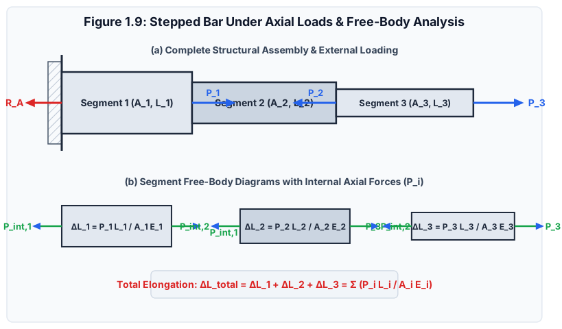
When an axially loaded member consists of multiple segments with differing cross-sectional areas (Ai), lengths (Li), or materials (Ei), and carries intermediate concentrated loads along its length:
Figure 1.9: Stepped prismatic bar with intermediate axial forces showing segment-by-segment free-body diagrams (FBD) and internal force equilibrium.
2.1 The Free-Body Diagram (FBD) Sectioning Technique
[!IMPORTANT]
Golden Rule of Internal Forces: Never use the external applied forces directly in the formula AEPL. The force Pi acting on segment i must be obtained by passing an imaginary cutting plane through segment i and establishing static equilibrium (∑Fx=0) for the isolated portion to either the left or the right of the cut.
For a bar comprising n discrete segments:
ΔLtotal=i=1∑nΔLi=i=1∑nAiEiPiLi
If segment i is in tension (Pi>0): ΔLi is positive (elongation).
If segment i is in compression (Pi<0): ΔLi is negative (contraction).
3. Mathematical Derivations: Elongation Under Self-Weight
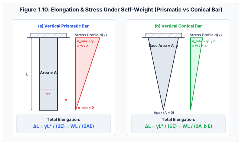
In deep boreholes, tall mine hoists, suspension bridge main cables, and vertical structural columns, the weight of the member itself produces significant axial elongation and stress.
Figure 1.10: Engineering comparison of vertical prismatic and conical bars under self-weight, showing internal normal stress distributions and total elongations.
3.1 Vertical Prismatic Bar Under Self-Weight
Consider a uniform prismatic bar of length L, cross-sectional area A, Young's modulus E, and mass density ρ (unit weight γ=ρg). The total weight of the bar is W=γAL.
Step 1: Internal Normal Force at Height x
Choose coordinate x measured upward from the bottom free tip (x=0):
The internal tensile force P(x) at any section x supports only the weight of the bar portion lying below that section:
P(x)=γ⋅A⋅x
Step 2: Normal Stress Distribution
σ(x)=AP(x)=γx
At the bottom free tip (x=0): σmin=0.
At the top fixed support (x=L):
σmax=γL=AW
The stress distribution varies linearly from zero at the bottom to a maximum at the top support.
Step 3: Integration for Total Elongation
The elongation of an infinitesimal element of length dx is dδ=AEP(x)dx=Eγxdx.
Integrating over the entire length from x=0 to x=L:
ΔL=∫0LEγxdx=Eγ[2x2]0L=2EγL2
Since γ=ALW:
ΔL=2E(ALW)L2=2AEWL
[!NOTE]
Fundamental Theorem of Self-Weight:
The elongation of a uniform vertical bar hanging under its own weight (2AEWL) is exactly half (50%) of the elongation produced by an external concentrated force equal to the total weight W applied at its bottom tip (AEWL).
3.2 Vertical Conical Bar Under Self-Weight
Consider a right circular cone of length L, base diameter D at the top fixed support, and apex at the bottom free tip (x=0).
Step 1: Geometry at Distance x from the Apex
At any section at height x from the apex:
Diameter: d(x)=LDx
Cross-sectional area:
A(x)=4π[d(x)]2=4π(LD)2x2
Step 2: Weight of the Conical Portion Below Section x
The volume of a cone of height x and base area A(x) is V(x)=31A(x)x.
Therefore, the weight supported at section x is:
P(x)=γ⋅V(x)=31γA(x)x
Step 3: Normal Stress Distribution
σ(x)=A(x)P(x)=A(x)31γA(x)x=31γx
Notice that the area A(x) cancels out! The normal stress varies linearly with x:
At the apex (x=0): σ=0.
At the top base (x=L):
σmax=31γL
Since the total weight of the cone is W=31γAbaseL⟹σmax=AbaseW.
Step 4: Total Elongation
ΔL=∫0LEσ(x)dx=∫0L3Eγxdx=3Eγ[2x2]0L=6EγL2
Expressed in terms of total weight W=31γAbaseL:
ΔL=2AbaseEWL
[!IMPORTANT]
Comparison of Self-Weight Elongations:
For a conical bar and a prismatic bar of the same length L and same material (γ,E):
ΔLprismaticΔLconical=2EγL26EγL2=31≈33.33%
The conical bar elongates by exactly one-third of the prismatic bar under self-weight!
4. Mathematical Derivations: Linearly Tapering Bars Under Axial Load P
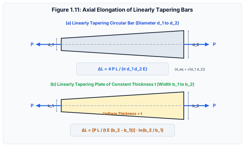
In structural design, members are frequently tapered to optimize material efficiency and reduce dead weight.
Figure 1.11: Linearly tapering circular bar and rectangular plate of uniform thickness under axial tensile load P.
4.1 Circular Linearly Tapering Bar
Consider a circular bar of length L whose diameter varies linearly from d1 at x=0 to d2 at x=L subjected to an axial tensile force P.
Step 1: Geometric Function for Diameter d(x)
d(x)=d1+(Ld2−d1)x
The cross-sectional area at distance x is:
A(x)=4π[d(x)]2=4π[d1+(Ld2−d1)x]2
Step 2: Integration for Total Elongation
ΔL=∫0LA(x)EPdx=πE4P∫0L[d1+(Ld2−d1)x]2dx
Let u=d1+(Ld2−d1)x⟹du=(Ld2−d1)dx⟹dx=d2−d1Ldu.
Limits of integration: at x=0⟹u=d1; at x=L⟹u=d2.
In heavy hanging cables, deep-sea risers, and chimney stacks, a prismatic bar is wasteful because the stress at the bottom is nearly zero while the top is heavily stressed.
A Bar of Uniform Strength is tapered such that the normal stress under self-weight plus external end load P0 is constant and equal to allowable working stress σ across every single cross-section.
5.1 Derivation of Cross-Sectional Area Function A(x)
Let x be measured downward from the top support (or upward from bottom load P0).
Measuring x upward from bottom end (x=0 where area is A0=P0/σ):
Consider an element of length dx at distance x:
Upward normal force on top face: P+dP=σ(A+dA)
Downward normal force on bottom face: P=σA
Downward weight of element: dW=γAdx
Equilibrium of the infinitesimal element:
(P+dP)−P−dW=0⟹σdA−γAdx=0AdA=σγdx
Integrating both sides from x=0 (where A=A0) to height x:
∫A0A(x)AdA=σγ∫0xdx⟹ln(A0A(x))=σγx
Exponentiating both sides:
A(x)=A0eσγx
where:
A0=σP0 is the minimum cross-sectional area at the bottom tip.
σ is the uniform constant working stress throughout the bar.
γ is the unit weight of the material.
6. Step-by-Step Solved Numerical Examples
Example 4.1: Stepped Bar under Multiple Intermediate Loads (GATE CE Level)
Problem Statement:
A steel bar firmly anchored to a rigid wall at support A consists of three prismatic segments as shown:
Segment AB: Length L1=500 mm, Area A1=1000 mm2
Segment BC: Length L2=400 mm, Area A2=500 mm2
Segment CD: Length L3=300 mm, Area A3=250 mm2
Modulus of Elasticity: E=200 GPa=2×10⁵ N/mm2
External axial forces applied at the junctions:
At junction B: PB=120 kN directed to the right (+x)
At junction C: PC=80 kN directed to the left (−x)
At free tip D: PD=50 kN directed to the right (+x)
Calculate:
The support reaction RA at the fixed anchor wall.
The internal axial force and normal stress in each of the three segments.
The displacement of junction B, junction C, and free tip D.
Step-by-Step Solution:
Overall Static Equilibrium (∑Fx=0):
Assume reaction RA acts to the left (−x):
−RA+PB−PC+PD=0−RA+120−80+50=0⟹RA=90 kN(directed to the left, tension at wall)
Internal Axial Force Determination by FBD Sectioning:
Segment CD (Cut between C and D, look to right):
To balance PD=50 kN pulling right:
P3=+50 kN=+50,000 N(Tension)
Segment BC (Cut between B and C, look to right):
Sum of forces to the right of cut: −PC+PD=−80+50=−30 kN.
To balance this, internal force on segment BC is:
P2=−30 kN=−30,000 N(Compression)
Segment AB (Cut between A and B, look to right):
Sum of forces to the right of cut: +PB−PC+PD=120−80+50=+90 kN.
P1=+90 kN=+90,000 N(Tension)Check against wall reaction:P1=RA=90 kN (Verified exact).
Segment 1:ΔL1=(1000 mm2)×(200,000 N/mm2)(+90,000 N)×(500 mm)=200,000,00045,000,000=+0.225 mm
Segment 2:ΔL2=(500 mm2)×(200,000 N/mm2)(−30,000 N)×(400 mm)=100,000,000−12,000,000=−0.120 mm
Segment 3:ΔL3=(250 mm2)×(200,000 N/mm2)(+50,000 N)×(300 mm)=50,000,00015,000,000=+0.300 mm
Displacements of Junctions:
Displacement of B: δB=ΔL1=+0.225 mm (to the right)
Displacement of C: δC=δB+ΔL2=+0.225−0.120=+0.105 mm (to the right)
Displacement of D (Tip): δD=δC+ΔL3=+0.105+0.300=+0.405 mm (to the right)
Independent Recalculation Check: ΔLtotal=0.225−0.120+0.300=+0.405 mm. Exact match.
Example 4.2: Tapering Circular Rod vs Arithmetic Mean Approximation (UPSC ESE Level)
Problem Statement:
A linearly tapering circular steel bar of length L=1000 mm has end diameters d1=20 mm and d2=40 mm. It is subjected to an axial pull of P=30 kN. Take E=200 GPa.
Compute the exact elongation (ΔLexact) using the derived tapering formula.
An engineer estimates the elongation by replacing the tapering bar with an equivalent prismatic bar having a diameter equal to the arithmetic mean (davg=2d1+d2). Compute this approximate elongation (ΔLapprox).
Determine the percentage error in the approximation.
Step-by-Step Solution:
Exact Elongation:
ΔLexact=πd1d2E4PLΔLexact=π×(20 mm)×(40 mm)×(200,000 N/mm2)4×(30,000 N)×(1000 mm)Numerator=120,000,000Denominator=π×800×200,000=160,000,000π≈502,654,824.57ΔLexact=502,654,824.57120,000,000=0.238732 mm≈0.2387 mm
Approximate Elongation using Arithmetic Mean Diameter (davg):
davg=220+40=30 mm
Area: Aavg=4π(30)2=225π≈706.8583 mm2.
ΔLapprox=AavgEPL=(225π)×200,00030,000×1000=45,000,000π30,000,000=3π2≈0.212207 mm
Critical Insight:
The arithmetic mean approximation underestimates the true elongation by 11.11%!
Why? Because flexibility depends on 1/d2. The thinner end (20 mm) deforms substantially more than the thicker end (40 mm), so taking an arithmetic average of diameter drastically underweights the flexible thin end.
Example 4.3: Vertical Steel Drill Pipe under Self-Weight and End Hook Load (SSC JE / State AE)
Problem Statement:
A vertical steel well drill pipe has length L=500 m, cross-sectional area A=4000 mm2, and unit weight γ=78.5 kN/m3=7.85×10−5 N/mm3. It carries a concentrated hook load of P0=120 kN at its bottom end. Take E=200 GPa=2×10⁵ N/mm2.
Calculate:
The total weight (W) of the drill pipe.
The total elongation (ΔL) of the drill pipe due to combined self-weight and bottom hook load.
The maximum tensile stress (σmax) and its location.
Step-by-Step Solution:
Total Weight of the Pipe (W):
Length L=500 m=500,000 mm.
Volume V=A×L=4000 mm2×500,000 mm=2×109 mm3=2.0 m3.
W=γ×V=(78.5 kN/m3)×(2.0 m3)=157.0 kN=157,000 N
Total Combined Elongation (ΔL):
By superposition: ΔL=ΔLself-weight+ΔLhook load.
Self-weight contribution:ΔLself-weight=2AEWL=2×(4000 mm2)×(200,000 N/mm2)(157,000 N)×(500,000 mm)=1,600,000,00078,500,000,000=49.0625 mm
Total Elongation:ΔL=49.0625 mm+75.000 mm=124.0625 mm≈124.06 mm
Maximum Tensile Stress (σmax):
Occurs at the top fixed suspension collar (x=L), where it must support the entire pipe weight plus the bottom hook load:
Verification Check: At bottom tip (x=0): σmin=AP0=4000120,000=30.0 MPa. Stress increases linearly from 30.0 MPa at bottom to 69.25 MPa at top. Recalculations exact.
7. Common Pitfalls & Competitive Exam Traps
[!WARNING]
Trap 1: Forgetting that Self-Weight Elongation is 2AEWL, NOT AEWL
In SSC JE and RRB JE objective questions, options almost always include both AEWL and 2AEWL.
Remember: Internal force under self-weight varies linearly from 0 to W. The average force is W/2, producing exactly half the elongation of an end load.
[!WARNING]
Trap 2: The Conical Bar Elongation Ratio
When comparing a conical bar to a prismatic bar under self-weight:
If compared based on same length and top base area: ΔLcone=31ΔLprismatic=6EγL2.
If compared based on same total weight W: ΔLcone=2AbEWL=ΔLprismatic!
Pay meticulous attention to whether the question states "same dimensions" or "same weight".
[!WARNING]
Trap 3: Arithmetic Mean vs Geometric Mean in Tapering Bars
In GATE NAT questions, if a problem asks for equivalent diameter deq, never use 2d1+d2. The exact equivalent diameter is d1d2.
8. Quick Revision Formula Box
Prismatic Bar under Point Load:ΔLStepped Bar Superposition:ΔLtotalPrismatic Bar under Self-Weight:ΔLConical Bar under Self-Weight:ΔLRatio (Conical to Prismatic, same L,γ):ΔLprismΔLconeCircular Tapering Bar:ΔLRectangular Tapering Plate (Const t):ΔLBar of Uniform Strength:A(x)=AEPL=i=1∑nAiEiPiLi=2EγL2=2AEWL=6EγL2=2AbaseEWL=31=πd1d2E4PL(deq=d1d2)=tE(b2−b1)PLln(b1b2)=A0eσγx
9. References & Source Literature
Gere, J. M., & Goodno, B. J. (2018). Mechanics of Materials, 9th Edition, Cengage Learning, Boston.
Timoshenko, S. P. (1953). History of Strength of Materials, McGraw-Hill, New York.
Punmia, B. C., Jain, A. K., & Jain, A. K. (2017). Mechanics of Materials, 15th Edition, Laxmi Publications, New Delhi.
Bhavikatti, S. S. (2019). Strength of Materials, 4th Edition, Vikas Publishing House, New Delhi.