SOM-02-04 Chapter 02 · Principal Stresses and Strains

Analysis of Strain, Strain Transformation & Strain Rosettes

In this chapter (5 topics)
On this page
  1. 1. Metadata & Syllabus Mapping
  2. Official Examination Syllabus Mapping
  3. 2. Introduction & Physical Mechanics
  4. Engineering Strain vs. Tensor Shear Strain
  5. ⚠️ The Golden Law of Strain Transformation
  6. 3. Mathematical Formulations & Derivations
  7. 3.1 Kinematic Derivation of Normal Strain on an Oblique Fiber (εθ)
  8. 3.2 Shear Strain Transformation Equation (γθ)
  9. 3.3 Principal Strains and Maximum In-Plane Shear Strain
  10. ⭐ The Crucial Engineering Factor of 2
  11. 3.4 Mohr's Circle of Strain
  12. 3.5 Strain Rosettes: Configurations & Data Reduction
  13. 3.6 Recovering Principal Stresses via Generalized Hooke's Law
  14. 4. Engineering Assumptions & Limitations
  15. 5. Technical Diagrams
  16. Diagram 1: 2D Strain Transformation Element & Kinematic Deformation
  17. Diagram 2: Strain Rosette Configurations & Stress Recovery
  18. 6. Solved Numerical Examples
  19. Example 4.1: Plane Strain Transformation & Mohr's Circle
  20. Example 4.2: 45° Rectangular Strain Rosette on Structural Steel
  21. Example 4.3: 60° Delta Rosette on an Aluminum Pressure Vessel
  22. 7. Practical & Field Engineering Applications
  23. 8. Comparative Analysis
  24. Stress Transformation vs. Strain Transformation
  25. Strain Rosette Configurations Comparison
  26. 9. Key Engineering Facts & Exam Takeaways
  27. 10. Common Pitfalls, Traps & Anti-Patterns
  28. 11. Standards & Code Provisions
  29. ASTM E251 (Standard Test Methods for Performance Characteristics of Metallic Bonded Resistance Strain-Gauges)
  30. ASTM E837 (Standard Test Method for Determining Residual Stresses by the Hole-Drilling Strain-Gage Method)
  31. IS 13916 (Code of Practice for Measurement of Strains in Concrete and Rock Structures)
  32. 12. Comprehensive Formula Box & Practice Problems
  33. Master Formula Summary
  34. Practice Problems

1. Metadata & Syllabus Mapping

Attribute Specification
Topic ID SOM-02-04
Module / Subject Subject 02: Strength of Materials (notes/strength_of_materials/)
Chapter Chapter 02: Principal Stresses and Strains (02_principal_stresses_and_strains)
Target Examinations GATE CE, UPSC ESE, SSC JE, RRB JE, State AE, State JE
Prerequisites SOM-01-01 (Stress and Strain), SOM-01-03 (Elastic Constants), SOM-02-01 (Stress Transformation), SOM-02-03 (Mohr's Circle)
Primary Code References ASTM E251 (Strain Gauge Testing), ASTM E837 (Residual Stress by Hole-Drilling), IS 13916
Verification Gate Level 1 through Level 7 Quality Standards

Official Examination Syllabus Mapping

Website note: this mapping is from the author’s notes. It has not been checked against the official notification for each examination; confirm the current syllabus with the examining body.

- GATE Civil Engineering: Solid Mechanics — Transformation of strain; Mohr's circle of strain; principal strains; maximum shear strain; strain rosettes (rectangular and delta rosettes); determination of principal stresses from strain measurements.
- UPSC ESE (Engineering Services): Paper-I Solid Mechanics — Analysis of plane strain; strain tensor vs engineering strain; Mohr's strain circle; electrical resistance strain gauges; strain rosette equations; calculation of stresses in thin walls and pressure vessels.
- SSC JE / RRB JE / State AE: Definition of principal strains; strain rosette types (45° and 60°); relation between engineering shear strain and tensor shear strain (γ = 2ε_xy); volumetric strain.

2. Introduction & Physical Mechanics

In experimental structural engineering and field monitoring of bridges, pressure vessels, and aerospace components, stress cannot be measured directly. No physical sensor exists that directly records force per unit area inside a solid material.

Instead, experimentalists measure surface displacements and normal strains using bonded electrical resistance strain gauges. By measuring normal strains along three independent directions at a single point (known as a strain rosette), engineers can reconstruct the complete 2D strain state (ϵx,ϵy,γxy)(\epsilon_x, \epsilon_y, \gamma_{xy}), compute the principal strains and directions, and then determine the true principal stresses via constitutive elasticity relations (Generalized Hooke's Law).

Engineering Strain vs. Tensor Shear Strain

A critical distinction must be maintained between engineering shear strain (γ\gamma) and tensor shear strain (ϵxy\epsilon_{xy}):

  • Engineering Shear Strain (γxy\gamma_{xy}): The total change in the right angle (90∘90^\circ angle) between two originally orthogonal line segments, measured in radians.
  • Tensor Shear Strain (ϵxy\epsilon_{xy}): The mathematical tensor component representing the mean angular rotation of the two line segments: ϵxy=12γxy(Eq. 4.1)\mathbf{\epsilon_{xy} = \frac{1}{2}\gamma_{xy}} \tag{Eq. 4.1}

⚠️ The Golden Law of Strain Transformation

All stress transformation formulas and Mohr's circle geometric constructions apply identically to strain transformations provided that every occurrence of normal stress σ\sigma is replaced by normal strain ϵ\epsilon, and every occurrence of shear stress τ\tau is replaced by half the engineering shear strain (γ2\frac{\gamma}{2} or tensor strain ϵxy\epsilon_{xy}).


3. Mathematical Formulations & Derivations

3.1 Kinematic Derivation of Normal Strain on an Oblique Fiber (ϵθ\epsilon_\theta)

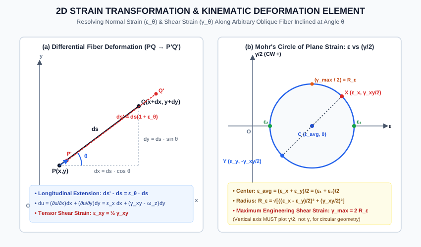
Consider an infinitesimal line segment PQPQ of length dsds inclined at an angle θ\theta counterclockwise from the xx-axis in a continuous 2D deformable medium.

The undeformed coordinate projections are:

dx=dscos⁡θ,dy=dssin⁡θ(Eq. 4.2)dx = ds \cos \theta, \quad dy = ds \sin \theta \tag{Eq. 4.2} ds2=dx2+dy2(Eq. 4.3)ds^2 = dx^2 + dy^2 \tag{Eq. 4.3}

Under 2D deformation, point P(x,y)P(x,y) displaces to P′(x+u,y+v)P'(x+u, y+v), and point Q(x+dx,y+dy)Q(x+dx, y+dy) displaces to Q′(x+dx+u+du,y+dy+v+dv)Q'(x+dx+u+du, y+dy+v+dv).
The differential displacement increments (du,dv)(du, dv) are given by Taylor series expansion:

du=∂u∂xdx+∂u∂ydy(Eq. 4.4a)du = \frac{\partial u}{\partial x}dx + \frac{\partial u}{\partial y}dy \tag{Eq. 4.4a} dv=∂v∂xdx+∂v∂ydy(Eq. 4.4b)dv = \frac{\partial v}{\partial x}dx + \frac{\partial v}{\partial y}dy \tag{Eq. 4.4b}

Recall the infinitesimal strain-displacement definitions:

ϵx=∂u∂x,ϵy=∂v∂y,γxy=∂u∂y+∂v∂x(Eq. 4.5)\epsilon_x = \frac{\partial u}{\partial x}, \quad \epsilon_y = \frac{\partial v}{\partial y}, \quad \gamma_{xy} = \frac{\partial u}{\partial y} + \frac{\partial v}{\partial x} \tag{Eq. 4.5}

The length of the deformed line segment P′Q′P'Q' (ds′ds') is:

(ds′)2=(dx+du)2+(dy+dv)2(ds')^2 = (dx + du)^2 + (dy + dv)^2 (ds′)2=(dx)2+2dxdu+(du)2+(dy)2+2dydv+(dv)2(ds')^2 = (dx)^2 + 2dx du + (du)^2 + (dy)^2 + 2dy dv + (dv)^2

For small deformations (ϵ≪1\epsilon \ll 1), second-order terms (du)2(du)^2 and (dv)2(dv)^2 are negligible:

(ds′)2≈ds2+2(dxdu+dydv)(Eq. 4.6)(ds')^2 \approx ds^2 + 2(dx du + dy dv) \tag{Eq. 4.6}

By definition of normal strain along line PQPQ:

ϵθ=ds′−dsds  ⟹  ds′=ds(1+ϵθ)\epsilon_\theta = \frac{ds' - ds}{ds} \implies ds' = ds(1 + \epsilon_\theta) (ds′)2=ds2(1+ϵθ)2≈ds2(1+2ϵθ)=ds2+2ϵθds2(Eq. 4.7)(ds')^2 = ds^2(1 + \epsilon_\theta)^2 \approx ds^2(1 + 2\epsilon_\theta) = ds^2 + 2\epsilon_\theta ds^2 \tag{Eq. 4.7}

Equating Eq. (4.6) and Eq. (4.7):

2ϵθds2=2(dxdu+dydv)  ⟹  ϵθ=dxdsduds+dydsdvds(Eq. 4.8)2\epsilon_\theta ds^2 = 2(dx du + dy dv) \implies \epsilon_\theta = \frac{dx}{ds}\frac{du}{ds} + \frac{dy}{ds}\frac{dv}{ds} \tag{Eq. 4.8}

Substitute dx/ds=cos⁡θdx / ds = \cos \theta, dy/ds=sin⁡θdy / ds = \sin \theta, and expansions for dudu and dvdv:

duds=∂u∂xcos⁡θ+∂u∂ysin⁡θ=ϵxcos⁡θ+∂u∂ysin⁡θ\frac{du}{ds} = \frac{\partial u}{\partial x}\cos \theta + \frac{\partial u}{\partial y}\sin \theta = \epsilon_x \cos \theta + \frac{\partial u}{\partial y}\sin \theta dvds=∂v∂xcos⁡θ+∂v∂ysin⁡θ=∂v∂xcos⁡θ+ϵysin⁡θ\frac{dv}{ds} = \frac{\partial v}{\partial x}\cos \theta + \frac{\partial v}{\partial y}\sin \theta = \frac{\partial v}{\partial x}\cos \theta + \epsilon_y \sin \theta

Plugging into Eq. (4.8):

ϵθ=cos⁡θ(ϵxcos⁡θ+∂u∂ysin⁡θ)+sin⁡θ(∂v∂xcos⁡θ+ϵysin⁡θ)\epsilon_\theta = \cos \theta\left(\epsilon_x \cos \theta + \frac{\partial u}{\partial y}\sin \theta\right) + \sin \theta\left(\frac{\partial v}{\partial x}\cos \theta + \epsilon_y \sin \theta\right) ϵθ=ϵxcos⁡2θ+ϵysin⁡2θ+(∂u∂y+∂v∂x)sin⁡θcos⁡θ\epsilon_\theta = \epsilon_x \cos^2 \theta + \epsilon_y \sin^2 \theta + \left(\frac{\partial u}{\partial y} + \frac{\partial v}{\partial x}\right)\sin \theta \cos \theta ϵθ=ϵxcos⁡2θ+ϵysin⁡2θ+γxysin⁡θcos⁡θ(Eq. 4.9)\mathbf{\epsilon_\theta = \epsilon_x \cos^2 \theta + \epsilon_y \sin^2 \theta + \gamma_{xy}\sin \theta \cos \theta} \tag{Eq. 4.9}

Using the double-angle trigonometric identities:

cos⁡2θ=1+cos⁡2θ2,sin⁡2θ=1−cos⁡2θ2,sin⁡θcos⁡θ=sin⁡2θ2\cos^2 \theta = \frac{1 + \cos 2\theta}{2}, \quad \sin^2 \theta = \frac{1 - \cos 2\theta}{2}, \quad \sin \theta \cos \theta = \frac{\sin 2\theta}{2}

We obtain the canonical Normal Strain Transformation Equation:

ϵθ=(ϵx+ϵy2)+(ϵx−ϵy2)cos⁡2θ+(γxy2)sin⁡2θ(Eq. 4.10)\mathbf{\epsilon_\theta = \left(\frac{\epsilon_x + \epsilon_y}{2}\right) + \left(\frac{\epsilon_x - \epsilon_y}{2}\right)\cos 2\theta + \left(\frac{\gamma_{xy}}{2}\right)\sin 2\theta} \tag{Eq. 4.10}

3.2 Shear Strain Transformation Equation (γθ\gamma_\theta)

By evaluating the change in right angle between two orthogonal fibers inclined at θ\theta and θ+90∘\theta + 90^\circ:

γθ2=−(ϵx−ϵy2)sin⁡2θ+(γxy2)cos⁡2θ(Eq. 4.11)\mathbf{\frac{\gamma_\theta}{2} = -\left(\frac{\epsilon_x - \epsilon_y}{2}\right)\sin 2\theta + \left(\frac{\gamma_{xy}}{2}\right)\cos 2\theta} \tag{Eq. 4.11} γθ=−(ϵx−ϵy)sin⁡2θ+γxycos⁡2θ(Eq. 4.12)\mathbf{\gamma_\theta = -(\epsilon_x - \epsilon_y)\sin 2\theta + \gamma_{xy}\cos 2\theta} \tag{Eq. 4.12}

Notice the direct one-to-one mathematical isomorphism with the stress transformation equations:

σ⟷ϵ\sigma \longleftrightarrow \epsilon τ⟷γ2=ϵxy\tau \longleftrightarrow \frac{\gamma}{2} = \epsilon_{xy}

3.3 Principal Strains and Maximum In-Plane Shear Strain

1. Principal Strain Planes (γθ=0\gamma_\theta = 0)

Equating shear strain in Eq. (4.11) to zero:

tan⁡2θp=γxyϵx−ϵy=γxy2ϵx−ϵy2(Eq. 4.13)\mathbf{\tan 2\theta_p = \frac{\gamma_{xy}}{\epsilon_x - \epsilon_y} = \frac{\frac{\gamma_{xy}}{2}}{\frac{\epsilon_x - \epsilon_y}{2}}} \tag{Eq. 4.13}

Because tan⁡2θp\tan 2\theta_p has two roots separated by 180∘180^\circ, the two principal strain axes are mutually perpendicular:

θp2=θp1+90∘(Eq. 4.14)\theta_{p2} = \theta_{p1} + 90^\circ \tag{Eq. 4.14}

2. Magnitudes of Principal Strains (ϵ1,ϵ2\epsilon_1, \epsilon_2)

Substituting cos⁡2θp\cos 2\theta_p and sin⁡2θp\sin 2\theta_p into Eq. (4.10):

ϵ1,2=(ϵx+ϵy2)±(ϵx−ϵy2)2+(γxy2)2(Eq. 4.15)\mathbf{\epsilon_{1,2} = \left(\frac{\epsilon_x + \epsilon_y}{2}\right) \pm \sqrt{\left(\frac{\epsilon_x - \epsilon_y}{2}\right)^2 + \left(\frac{\gamma_{xy}}{2}\right)^2}} \tag{Eq. 4.15}

Defining the Average Normal Strain:

ϵavg=ϵx+ϵy2(Eq. 4.16)\epsilon_{\text{avg}} = \frac{\epsilon_x + \epsilon_y}{2} \tag{Eq. 4.16}

and the Strain Circle Radius:

Rϵ=(ϵx−ϵy2)2+(γxy2)2(Eq. 4.17)R_\epsilon = \sqrt{\left(\frac{\epsilon_x - \epsilon_y}{2}\right)^2 + \left(\frac{\gamma_{xy}}{2}\right)^2} \tag{Eq. 4.17}

We have:

ϵ1=ϵavg+Rϵ(Major Principal Strain)(Eq. 4.18a)\mathbf{\epsilon_1 = \epsilon_{\text{avg}} + R_\epsilon} \quad (\text{Major Principal Strain}) \tag{Eq. 4.18a} ϵ2=ϵavg−Rϵ(Minor Principal Strain)(Eq. 4.18b)\mathbf{\epsilon_2 = \epsilon_{\text{avg}} - R_\epsilon} \quad (\text{Minor Principal Strain}) \tag{Eq. 4.18b}

3. Maximum In-Plane Shear Strain (γmax⁡\gamma_{\max})

The maximum value of the tensor shear strain is equal to the radius RϵR_\epsilon:

(γmax⁡2)=Rϵ\left(\frac{\gamma_{\max}}{2}\right) = R_\epsilon

Therefore, the maximum engineering shear strain is:

γmax⁡,in-plane=2Rϵ=2(ϵx−ϵy2)2+(γxy2)2=ϵ1−ϵ2(Eq. 4.19)\mathbf{\gamma_{\max, \text{in-plane}} = 2 R_\epsilon = 2\sqrt{\left(\frac{\epsilon_x - \epsilon_y}{2}\right)^2 + \left(\frac{\gamma_{xy}}{2}\right)^2} = \epsilon_1 - \epsilon_2} \tag{Eq. 4.19}

⭐ The Crucial Engineering Factor of 2

In stress analysis, τmax⁡=Rσ=σ1−σ22\tau_{\max} = R_\sigma = \frac{\sigma_1 - \sigma_2}{2}.
In strain analysis, the radius is Rϵ=ϵ1−ϵ22R_\epsilon = \frac{\epsilon_1 - \epsilon_2}{2}, but the maximum engineering shear strain is γmax⁡=2Rϵ=ϵ1−ϵ2\gamma_{\max} = 2 R_\epsilon = \epsilon_1 - \epsilon_2! This is one of the most frequently tested traps in GATE and ESE.

4. Strain Invariant (First Invariant of Strain)

I1,ϵ=ϵx+ϵy=ϵ1+ϵ2=Constant(Eq. 4.20)\mathbf{I_{1,\epsilon} = \epsilon_x + \epsilon_y = \epsilon_1 + \epsilon_2 = \text{Constant}} \tag{Eq. 4.20}

3.4 Mohr's Circle of Strain

By eliminating 2θ2\theta between Eq. (4.10) and Eq. (4.11):

(ϵθ−ϵavg)2+(γθ2)2=Rϵ2(Eq. 4.21)\mathbf{\left(\epsilon_\theta - \epsilon_{\text{avg}}\right)^2 + \left(\frac{\gamma_\theta}{2}\right)^2 = R_\epsilon^2} \tag{Eq. 4.21}

Construction Rules:

  • Horizontal Axis: Normal strain ϵ\epsilon (positive extension right, contraction left).
  • Vertical Axis: Half of engineering shear strain γ2\frac{\gamma}{2} (clockwise shear positive upward).
  • Center: C=(ϵavg,0)=(ϵx+ϵy2,0)C = (\epsilon_{\text{avg}}, 0) = \left(\frac{\epsilon_x + \epsilon_y}{2}, 0\right).
  • Radius: Rϵ=(ϵx−ϵy2)2+(γxy2)2=ϵ1−ϵ22R_\epsilon = \sqrt{\left(\frac{\epsilon_x - \epsilon_y}{2}\right)^2 + \left(\frac{\gamma_{xy}}{2}\right)^2} = \frac{\epsilon_1 - \epsilon_2}{2}.
  • Reference Coordinates:
    • Face xx: X=(ϵx,+γxy2)X = \left(\epsilon_x, +\frac{\gamma_{xy}}{2}\right)
    • Face yy: Y=(ϵy,−γxy2)Y = \left(\epsilon_y, -\frac{\gamma_{xy}}{2}\right)

Line XYXY forms the reference diameter passing through center CC.


3.5 Strain Rosettes: Configurations & Data Reduction

A strain rosette is an arrangement of three electrical resistance strain gauges bonded close together on the surface of a component. Each gauge measures the normal strain along its longitudinal axis.

Let the three gauges be oriented at angles θa,θb,θc\theta_a, \theta_b, \theta_c relative to the xx-axis. From Eq. (4.9), the recorded strains satisfy the system of 3 linear equations:

ϵa=ϵxcos⁡2θa+ϵysin⁡2θa+γxysin⁡θacos⁡θa(Eq. 4.22a)\epsilon_a = \epsilon_x \cos^2 \theta_a + \epsilon_y \sin^2 \theta_a + \gamma_{xy}\sin \theta_a \cos \theta_a \tag{Eq. 4.22a} ϵb=ϵxcos⁡2θb+ϵysin⁡2θb+γxysin⁡θbcos⁡θb(Eq. 4.22b)\epsilon_b = \epsilon_x \cos^2 \theta_b + \epsilon_y \sin^2 \theta_b + \gamma_{xy}\sin \theta_b \cos \theta_b \tag{Eq. 4.22b} ϵc=ϵxcos⁡2θc+ϵysin⁡2θc+γxysin⁡θccos⁡θc(Eq. 4.22c)\epsilon_c = \epsilon_x \cos^2 \theta_c + \epsilon_y \sin^2 \theta_c + \gamma_{xy}\sin \theta_c \cos \theta_c \tag{Eq. 4.22c}

Solving this 3×33 \times 3 system yields the three unknowns: ϵx,ϵy,γxy\epsilon_x, \epsilon_y, \gamma_{xy}.


1. The 45∘45^\circ Rectangular Rosette

Gauges are oriented at:

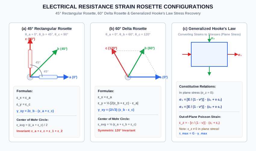
θa=0∘,θb=45∘,θc=90∘\theta_a = 0^\circ, \quad \theta_b = 45^\circ, \quad \theta_c = 90^\circ
  • For Gauge aa (θ=0∘\theta = 0^\circ):

    ϵa=ϵxcos⁡20∘+ϵysin⁡20∘+γxysin⁡0∘cos⁡0∘  ⟹  ϵx=ϵa(Eq. 4.23a)\epsilon_a = \epsilon_x \cos^2 0^\circ + \epsilon_y \sin^2 0^\circ + \gamma_{xy}\sin 0^\circ \cos 0^\circ \implies \mathbf{\epsilon_x = \epsilon_a} \tag{Eq. 4.23a}
  • For Gauge cc (θ=90∘\theta = 90^\circ):

    ϵc=ϵxcos⁡290∘+ϵysin⁡290∘+γxysin⁡90∘cos⁡90∘  ⟹  ϵy=ϵc(Eq. 4.23b)\epsilon_c = \epsilon_x \cos^2 90^\circ + \epsilon_y \sin^2 90^\circ + \gamma_{xy}\sin 90^\circ \cos 90^\circ \implies \mathbf{\epsilon_y = \epsilon_c} \tag{Eq. 4.23b}
  • For Gauge bb (θ=45∘\theta = 45^\circ):

    ϵb=ϵxcos⁡245∘+ϵysin⁡245∘+γxysin⁡45∘cos⁡45∘=ϵx2+ϵy2+γxy2\epsilon_b = \epsilon_x \cos^2 45^\circ + \epsilon_y \sin^2 45^\circ + \gamma_{xy}\sin 45^\circ \cos 45^\circ = \frac{\epsilon_x}{2} + \frac{\epsilon_y}{2} + \frac{\gamma_{xy}}{2} 2ϵb=ϵx+ϵy+γxy=ϵa+ϵc+γxy2\epsilon_b = \epsilon_x + \epsilon_y + \gamma_{xy} = \epsilon_a + \epsilon_c + \gamma_{xy} γxy=2ϵb−(ϵa+ϵc)(Eq. 4.23c)\mathbf{\gamma_{xy} = 2\epsilon_b - (\epsilon_a + \epsilon_c)} \tag{Eq. 4.23c}

2. The 60∘60^\circ Delta (Equilateral) Rosette

Gauges are oriented symmetrically at:

θa=0∘,θb=60∘,θc=120∘\theta_a = 0^\circ, \quad \theta_b = 60^\circ, \quad \theta_c = 120^\circ
  • For Gauge aa (θ=0∘\theta = 0^\circ):

    ϵx=ϵa(Eq. 4.24a)\mathbf{\epsilon_x = \epsilon_a} \tag{Eq. 4.24a}
  • For Gauge bb (θ=60∘\theta = 60^\circ, cos⁡60∘=1/2\cos 60^\circ = 1/2, sin⁡60∘=3/2\sin 60^\circ = \sqrt{3}/2):

    ϵb=ϵx(14)+ϵy(34)+γxy(34)(Eq. 4.24b)\epsilon_b = \epsilon_x \left(\frac{1}{4}\right) + \epsilon_y \left(\frac{3}{4}\right) + \gamma_{xy}\left(\frac{\sqrt{3}}{4}\right) \tag{Eq. 4.24b}
  • For Gauge cc (θ=120∘\theta = 120^\circ, cos⁡120∘=−1/2\cos 120^\circ = -1/2, sin⁡120∘=3/2\sin 120^\circ = \sqrt{3}/2):

    ϵc=ϵx(14)+ϵy(34)−γxy(34)(Eq. 4.24c)\epsilon_c = \epsilon_x \left(\frac{1}{4}\right) + \epsilon_y \left(\frac{3}{4}\right) - \gamma_{xy}\left(\frac{\sqrt{3}}{4}\right) \tag{Eq. 4.24c}
  • Adding Eq. (4.24b) and Eq. (4.24c):

    ϵb+ϵc=ϵx2+3ϵy2=ϵa2+3ϵy2\epsilon_b + \epsilon_c = \frac{\epsilon_x}{2} + \frac{3\epsilon_y}{2} = \frac{\epsilon_a}{2} + \frac{3\epsilon_y}{2} 3ϵy2=(ϵb+ϵc)−ϵa2  ⟹  ϵy=2(ϵb+ϵc)−ϵa3(Eq. 4.24d)\frac{3\epsilon_y}{2} = (\epsilon_b + \epsilon_c) - \frac{\epsilon_a}{2} \implies \mathbf{\epsilon_y = \frac{2(\epsilon_b + \epsilon_c) - \epsilon_a}{3}} \tag{Eq. 4.24d}
  • Subtracting Eq. (4.24c) from Eq. (4.24b):

    ϵb−ϵc=234γxy=32γxy\epsilon_b - \epsilon_c = \frac{2\sqrt{3}}{4}\gamma_{xy} = \frac{\sqrt{3}}{2}\gamma_{xy} γxy=2(ϵb−ϵc)3(Eq. 4.24e)\mathbf{\gamma_{xy} = \frac{2(\epsilon_b - \epsilon_c)}{\sqrt{3}}} \tag{Eq. 4.24e}
  • Average Normal Strain for Delta Rosette:

    ϵavg=ϵx+ϵy2=ϵa+ϵb+ϵc3(Eq. 4.24f)\mathbf{\epsilon_{\text{avg}} = \frac{\epsilon_x + \epsilon_y}{2} = \frac{\epsilon_a + \epsilon_b + \epsilon_c}{3}} \tag{Eq. 4.24f}

3.6 Recovering Principal Stresses via Generalized Hooke's Law

Once principal strains (ϵ1,ϵ2)(\epsilon_1, \epsilon_2) are determined from rosette measurements, how do we find the principal stresses?

Because strain rosettes are mounted on the free surface of a structural element:

σ3=σz=0(State of Plane Stress)(Eq. 4.25)\sigma_3 = \sigma_z = 0 \quad (\text{State of Plane Stress}) \tag{Eq. 4.25}

Under Generalized Hooke's Law for plane stress:

ϵ1=σ1E−νσ2E(Eq. 4.26a)\epsilon_1 = \frac{\sigma_1}{E} - \nu \frac{\sigma_2}{E} \tag{Eq. 4.26a} ϵ2=σ2E−νσ1E(Eq. 4.26b)\epsilon_2 = \frac{\sigma_2}{E} - \nu \frac{\sigma_1}{E} \tag{Eq. 4.26b}

Multiplying Eq. (4.26b) by ν\nu and adding to Eq. (4.26a):

ϵ1+νϵ2=σ1E(1−ν2)  ⟹  σ1=E1−ν2(ϵ1+νϵ2)(Eq. 4.27a)\epsilon_1 + \nu \epsilon_2 = \frac{\sigma_1}{E}(1 - \nu^2) \implies \mathbf{\sigma_1 = \frac{E}{1 - \nu^2}\left(\epsilon_1 + \nu \epsilon_2\right)} \tag{Eq. 4.27a}

Similarly, for the minor principal stress:

σ2=E1−ν2(ϵ2+νϵ1)(Eq. 4.27b)\mathbf{\sigma_2 = \frac{E}{1 - \nu^2}\left(\epsilon_2 + \nu \epsilon_1\right)} \tag{Eq. 4.27b}

Out-of-Plane Poisson Strain (ϵz\epsilon_z):

Even though σz=0\sigma_z = 0, the out-of-plane normal strain is NOT ZERO:

ϵz=−νE(σ1+σ2)=−ν1−ν(ϵ1+ϵ2)=−ν1−ν(ϵx+ϵy)(Eq. 4.28)\mathbf{\epsilon_z = -\frac{\nu}{E}(\sigma_1 + \sigma_2) = -\frac{\nu}{1 - \nu}\left(\epsilon_1 + \epsilon_2\right) = -\frac{\nu}{1 - \nu}\left(\epsilon_x + \epsilon_y\right)} \tag{Eq. 4.28}

Maximum Shear Stress Recovery:

τmax⁡,in-plane=σ1−σ22=E2(1+ν)(ϵ1−ϵ2)=G⋅γmax⁡(Eq. 4.29)\mathbf{\tau_{\max, \text{in-plane}} = \frac{\sigma_1 - \sigma_2}{2} = \frac{E}{2(1 + \nu)}(\epsilon_1 - \epsilon_2) = G \cdot \gamma_{\max}} \tag{Eq. 4.29}

4. Engineering Assumptions & Limitations

  1. Small Deformation Theory: Displacements and strain gradients are small (ϵ≪1\epsilon \ll 1), justifying the omission of quadratic terms (du)2,(dv)2(du)^2, (dv)^2.
  2. Homogeneous, Isotropic Elastic Solid: Hooke's Law inversion relies on uniform elastic modulus EE and Poisson's ratio ν\nu.
  3. Plane Stress Boundary Condition: The surface on which the rosette is bonded must be free of normal surface traction (σz=0\sigma_z = 0). If intense transverse contact pressure acts on the gauge, 3D constitutive equations must be applied.
  4. Point Collocation Assumption: The three gauge filaments occupy distinct physical footprints (typically separated by 2 to 5 mm2\text{ to }5\text{ mm}). It is assumed that strain gradients across this small gauge area are negligible.
  5. Transverse Sensitivity: Real foil strain gauges exhibit a small transverse sensitivity factor (kt≈0.5% to 2%k_t \approx 0.5\% \text{ to } 2\%), which must be calibrated out in precision aerospace applications.

5. Technical Diagrams

Diagram 1: 2D Strain Transformation Element & Kinematic Deformation

The vector diagram below illustrates differential fiber extension (ds→ds′ds \to ds'), the decomposition of displacement gradients, and the geometric construction of Mohr's Circle of Strain (ϵ\epsilon vs γ/2\gamma/2).

Strain Transformation Element

Diagram 2: Strain Rosette Configurations & Stress Recovery

The diagram below details the gauge geometry, algebraic extraction formulas, and Generalized Hooke's Law constitutive conversion for the 45∘45^\circ Rectangular Rosette and 60∘60^\circ Delta Rosette.

Strain Rosette Configurations

6. Solved Numerical Examples

Example 4.1: Plane Strain Transformation & Mohr's Circle

At a critical point on the outer surface of a machine housing, the plane strain components are:

  • ϵx=+400×10−6\epsilon_x = +400 \times 10^{-6} (+400 μϵ+400\ \mu\epsilon)
  • ϵy=−200×10−6\epsilon_y = -200 \times 10^{-6} (−200 μϵ-200\ \mu\epsilon)
  • γxy=+300×10−6 rad\gamma_{xy} = +300 \times 10^{-6}\text{ rad} (+300 μrad+300\ \mu\text{rad})

Determine:

  1. The center and radius of Mohr's circle of strain.
  2. The magnitudes of the major and minor principal strains (ϵ1,ϵ2\epsilon_1, \epsilon_2).
  3. The orientation of the principal strain axes (θp1,θp2\theta_{p1}, \theta_{p2}).
  4. The maximum in-plane engineering shear strain (γmax⁡\gamma_{\max}).
  5. The normal and engineering shear strain along a fiber inclined at θ=30∘\theta = 30^\circ counterclockwise to the xx-axis.
Given:
εx = +400 × 10^-6
εy = -200 × 10^-6
γxy = +300 × 10^-6 rad  => (γxy / 2) = +150 × 10^-6

Solution:

Step 1: Compute Center and Radius of Mohr's Circle of Strain

  • Center:

    ϵavg=ϵx+ϵy2=400+(−200)2×10−6=+100×10−6(+100 μϵ)\epsilon_{\text{avg}} = \frac{\epsilon_x + \epsilon_y}{2} = \frac{400 + (-200)}{2} \times 10^{-6} = \mathbf{+100 \times 10^{-6}}\quad (+100\ \mu\epsilon) C=(100×10−6,0)C = (100 \times 10^{-6}, 0)
  • Radius (RϵR_\epsilon):

    Rϵ=(ϵx−ϵy2)2+(γxy2)2=(400−(−200)2)2+1502×10−6R_\epsilon = \sqrt{\left(\frac{\epsilon_x - \epsilon_y}{2}\right)^2 + \left(\frac{\gamma_{xy}}{2}\right)^2} = \sqrt{\left(\frac{400 - (-200)}{2}\right)^2 + 150^2} \times 10^{-6} Rϵ=3002+1502×10−6=90000+22500×10−6=112500×10−6=335.41×10⁻⁶R_\epsilon = \sqrt{300^2 + 150^2} \times 10^{-6} = \sqrt{90000 + 22500} \times 10^{-6} = \sqrt{112500} \times 10^{-6} = \mathbf{335.41 \times 10^{-6}}

Step 2: Calculate Principal Strains

  • Major Principal Strain: ϵ1=ϵavg+Rϵ=100+335.41=+435.41×10⁻⁶(+435.41 μϵ)\epsilon_1 = \epsilon_{\text{avg}} + R_\epsilon = 100 + 335.41 = \mathbf{+435.41 \times 10^{-6}}\quad (+435.41\ \mu\epsilon)
  • Minor Principal Strain: ϵ2=ϵavg−Rϵ=100−335.41=−235.41×10⁻⁶(−235.41 μϵ)\epsilon_2 = \epsilon_{\text{avg}} - R_\epsilon = 100 - 335.41 = \mathbf{-235.41 \times 10^{-6}}\quad (-235.41\ \mu\epsilon)

Check Strain Invariant:

ϵ1+ϵ2=435.41+(−235.41)=+200 μϵ\epsilon_1 + \epsilon_2 = 435.41 + (-235.41) = +200\ \mu\epsilon ϵx+ϵy=400+(−200)=+200 μϵ(Confirmed)\epsilon_x + \epsilon_y = 400 + (-200) = +200\ \mu\epsilon\quad (\text{Confirmed})

Step 3: Principal Strain Orientations

tan⁡2θp=γxyϵx−ϵy=300400−(−200)=300600=0.50\tan 2\theta_p = \frac{\gamma_{xy}}{\epsilon_x - \epsilon_y} = \frac{300}{400 - (-200)} = \frac{300}{600} = 0.50 2θp1=arctan⁡(0.50)=26.565∘  ⟹  θp1=13.28∘ (Counterclockwise from x-axis)2\theta_{p1} = \arctan(0.50) = 26.565^\circ \implies \mathbf{\theta_{p1} = 13.28^\circ}\text{ (Counterclockwise from }x\text{-axis)} θp2=13.28∘+90∘=103.28∘\theta_{p2} = 13.28^\circ + 90^\circ = \mathbf{103.28^\circ}

Step 4: Maximum In-Plane Engineering Shear Strain

γmax⁡=2Rϵ=2(335.41×10⁻⁶)=670.82×10⁻⁶ rad(670.82 μrad)\gamma_{\max} = 2 R_\epsilon = 2(335.41 \times 10^{-6}) = \mathbf{670.82 \times 10^{-6}\text{ rad}}\quad (670.82\ \mu\text{rad})

Step 5: Strains on Plane Inclined at θ=30∘\theta = 30^\circ

ϵ30=ϵavg+(ϵx−ϵy2)cos⁡(60∘)+(γxy2)sin⁡(60∘)\epsilon_{30} = \epsilon_{\text{avg}} + \left(\frac{\epsilon_x - \epsilon_y}{2}\right)\cos(60^\circ) + \left(\frac{\gamma_{xy}}{2}\right)\sin(60^\circ) ϵ30=[100+300(0.5)+150(0.8660)]×10−6=[100+150+129.90]×10−6=+379.90×10⁻⁶\epsilon_{30} = [100 + 300(0.5) + 150(0.8660)] \times 10^{-6} = [100 + 150 + 129.90] \times 10^{-6} = \mathbf{+379.90 \times 10^{-6}} γ302=−(ϵx−ϵy2)sin⁡(60∘)+(γxy2)cos⁡(60∘)\frac{\gamma_{30}}{2} = -\left(\frac{\epsilon_x - \epsilon_y}{2}\right)\sin(60^\circ) + \left(\frac{\gamma_{xy}}{2}\right)\cos(60^\circ) γ302=[−300(0.8660)+150(0.5)]×10−6=[−259.81+75]×10−6=−184.81×10⁻⁶\frac{\gamma_{30}}{2} = [-300(0.8660) + 150(0.5)] \times 10^{-6} = [-259.81 + 75] \times 10^{-6} = -184.81 \times 10^{-6} γ30=2(−184.81×10⁻⁶)=−369.62×10⁻⁶ rad\gamma_{30} = 2(-184.81 \times 10^{-6}) = \mathbf{-369.62 \times 10^{-6}\text{ rad}}

Example 4.2: 45∘45^\circ Rectangular Strain Rosette on Structural Steel

A 45∘45^\circ rectangular strain rosette is mounted on the web of a structural steel I-beam (E=200 GPaE = 200\text{ GPa}, ν=0.30\nu = 0.30). The measured strains from the three gauges are:

  • Gauge aa (θa=0∘\theta_a = 0^\circ): ϵa=+500×10−6\epsilon_a = +500 \times 10^{-6}
  • Gauge bb (θb=45∘\theta_b = 45^\circ): ϵb=+350×10−6\epsilon_b = +350 \times 10^{-6}
  • Gauge cc (θc=90∘\theta_c = 90^\circ): ϵc=−100×10−6\epsilon_c = -100 \times 10^{-6}

Calculate:

  1. The in-plane strain components ϵx,ϵy,γxy\epsilon_x, \epsilon_y, \gamma_{xy}.
  2. The principal strains ϵ1,ϵ2\epsilon_1, \epsilon_2 and principal orientation θp\theta_p.
  3. The principal stresses σ1,σ2\sigma_1, \sigma_2 developed in the steel web.
  4. The out-of-plane normal strain ϵz\epsilon_z.
Given:
εa = +500 × 10^-6
εb = +350 × 10^-6
εc = -100 × 10^-6
E = 200 GPa = 200,000 MPa
ν = 0.30

Solution:

Step 1: Extract Strain Components

ϵx=ϵa=+500×10−6\epsilon_x = \epsilon_a = \mathbf{+500 \times 10^{-6}} ϵy=ϵc=−100×10−6\epsilon_y = \epsilon_c = \mathbf{-100 \times 10^{-6}} γxy=2ϵb−(ϵa+ϵc)=2(350)−(500+(−100))=700−400=+300×10−6 rad\gamma_{xy} = 2\epsilon_b - (\epsilon_a + \epsilon_c) = 2(350) - (500 + (-100)) = 700 - 400 = \mathbf{+300 \times 10^{-6}\text{ rad}}

Step 2: Compute Principal Strains

ϵavg=ϵx+ϵy2=500+(−100)2×10−6=+200×10−6\epsilon_{\text{avg}} = \frac{\epsilon_x + \epsilon_y}{2} = \frac{500 + (-100)}{2} \times 10^{-6} = +200 \times 10^{-6} ϵx−ϵy2=500−(−100)2×10−6=+300×10−6\frac{\epsilon_x - \epsilon_y}{2} = \frac{500 - (-100)}{2} \times 10^{-6} = +300 \times 10^{-6} γxy2=3002×10−6=+150×10−6\frac{\gamma_{xy}}{2} = \frac{300}{2} \times 10^{-6} = +150 \times 10^{-6} Rϵ=3002+1502×10−6=335.41×10⁻⁶R_\epsilon = \sqrt{300^2 + 150^2} \times 10^{-6} = 335.41 \times 10^{-6} ϵ1=ϵavg+Rϵ=200+335.41=+535.41×10⁻⁶\epsilon_1 = \epsilon_{\text{avg}} + R_\epsilon = 200 + 335.41 = \mathbf{+535.41 \times 10^{-6}} ϵ2=ϵavg−Rϵ=200−335.41=−135.41×10⁻⁶\epsilon_2 = \epsilon_{\text{avg}} - R_\epsilon = 200 - 335.41 = \mathbf{-135.41 \times 10^{-6}}

Orientation:

tan⁡2θp=γxyϵx−ϵy=300600=0.50  ⟹  θp1=13.28∘\tan 2\theta_p = \frac{\gamma_{xy}}{\epsilon_x - \epsilon_y} = \frac{300}{600} = 0.50 \implies \mathbf{\theta_{p1} = 13.28^\circ}

Step 3: Recover Principal Stresses via Hooke's Law (Plane Stress)

1−ν2=1−0.302=1−0.09=0.911 - \nu^2 = 1 - 0.30^2 = 1 - 0.09 = 0.91 E1−ν2=200,000 MPa0.91≈219,780.22 MPa\frac{E}{1 - \nu^2} = \frac{200,000\text{ MPa}}{0.91} \approx 219,780.22\text{ MPa}
  • Major Principal Stress:

    σ1=E1−ν2(ϵ1+νϵ2)=219,780.22×[535.41+0.30(−135.41)]×10−6\sigma_1 = \frac{E}{1 - \nu^2}\left(\epsilon_1 + \nu \epsilon_2\right) = 219,780.22 \times [535.41 + 0.30(-135.41)] \times 10^{-6} σ1=219,780.22×[535.41−40.623]×10−6=219,780.22×[494.787×10−6]=+108.74 MPa (Tension)\sigma_1 = 219,780.22 \times [535.41 - 40.623] \times 10^{-6} = 219,780.22 \times [494.787 \times 10^{-6}] = \mathbf{+108.74\text{ MPa}}\text{ (Tension)}
  • Minor Principal Stress:

    σ2=E1−ν2(ϵ2+νϵ1)=219,780.22×[−135.41+0.30(535.41)]×10−6\sigma_2 = \frac{E}{1 - \nu^2}\left(\epsilon_2 + \nu \epsilon_1\right) = 219,780.22 \times [-135.41 + 0.30(535.41)] \times 10^{-6} σ2=219,780.22×[−135.41+160.623]×10−6=219,780.22×[25.213×10−6]=+5.54 MPa (Tension)\sigma_2 = 219,780.22 \times [-135.41 + 160.623] \times 10^{-6} = 219,780.22 \times [25.213 \times 10^{-6}] = \mathbf{+5.54\text{ MPa}}\text{ (Tension)}

Step 4: Out-of-Plane Normal Strain (ϵz\epsilon_z)

ϵz=−ν1−ν(ϵx+ϵy)=−0.301−0.30(500−100)×10−6=−0.300.70(400×10−6)=−171.43×10⁻⁶\epsilon_z = -\frac{\nu}{1 - \nu}\left(\epsilon_x + \epsilon_y\right) = -\frac{0.30}{1 - 0.30}(500 - 100) \times 10^{-6} = -\frac{0.30}{0.70}(400 \times 10^{-6}) = \mathbf{-171.43 \times 10^{-6}}

Example 4.3: 60∘60^\circ Delta Rosette on an Aluminum Pressure Vessel

A 60∘60^\circ delta rosette mounted on an aluminum alloy cylinder (E=70 GPaE = 70\text{ GPa}, ν=0.33\nu = 0.33) records the following strain readings during hydrostatic pressure testing:

  • Gauge aa (θa=0∘\theta_a = 0^\circ): ϵa=+600×10−6\epsilon_a = +600 \times 10^{-6}
  • Gauge bb (θb=60∘\theta_b = 60^\circ): ϵb=+450×10−6\epsilon_b = +450 \times 10^{-6}
  • Gauge cc (θc=120∘\theta_c = 120^\circ): ϵc=+150×10−6\epsilon_c = +150 \times 10^{-6}

Determine:

  1. The strain components ϵx,ϵy,γxy\epsilon_x, \epsilon_y, \gamma_{xy}.
  2. The principal strains ϵ1,ϵ2\epsilon_1, \epsilon_2.
  3. The principal stresses σ1,σ2\sigma_1, \sigma_2.
  4. The maximum in-plane shear stress τmax⁡\tau_{\max} and verify consistency with the shear modulus GG.
Given:
εa = +600 × 10^-6
εb = +450 × 10^-6
εc = +150 × 10^-6
E = 70 GPa = 70,000 MPa
ν = 0.33

Solution:

Step 1: Extract Strain Components for Delta Rosette

ϵx=ϵa=+600×10−6\epsilon_x = \epsilon_a = \mathbf{+600 \times 10^{-6}} ϵy=2(ϵb+ϵc)−ϵa3=2(450+150)−6003×10−6=1200−6003×10−6=+200×10−6\epsilon_y = \frac{2(\epsilon_b + \epsilon_c) - \epsilon_a}{3} = \frac{2(450 + 150) - 600}{3} \times 10^{-6} = \frac{1200 - 600}{3} \times 10^{-6} = \mathbf{+200 \times 10^{-6}} γxy=2(ϵb−ϵc)3=2(450−150)3×10−6=6003×10−6=2003×10−6≈+346.41×10⁻⁶ rad\gamma_{xy} = \frac{2(\epsilon_b - \epsilon_c)}{\sqrt{3}} = \frac{2(450 - 150)}{\sqrt{3}} \times 10^{-6} = \frac{600}{\sqrt{3}} \times 10^{-6} = 200\sqrt{3} \times 10^{-6} \approx \mathbf{+346.41 \times 10^{-6}\text{ rad}}

Step 2: Compute Principal Strains

  • Average Strain:

    ϵavg=ϵa+ϵb+ϵc3=600+450+1503×10−6=+400×10−6\epsilon_{\text{avg}} = \frac{\epsilon_a + \epsilon_b + \epsilon_c}{3} = \frac{600 + 450 + 150}{3} \times 10^{-6} = +400 \times 10^{-6}
  • Difference terms:

    ϵx−ϵy2=600−2002×10−6=+200×10−6\frac{\epsilon_x - \epsilon_y}{2} = \frac{600 - 200}{2} \times 10^{-6} = +200 \times 10^{-6} γxy2=1003×10−6≈173.21×10⁻⁶\frac{\gamma_{xy}}{2} = 100\sqrt{3} \times 10^{-6} \approx 173.21 \times 10^{-6}
  • Radius:

    Rϵ=2002+(1003)2×10−6=40000+30000×10−6=70000×10−6=264.58×10⁻⁶R_\epsilon = \sqrt{200^2 + (100\sqrt{3})^2} \times 10^{-6} = \sqrt{40000 + 30000} \times 10^{-6} = \sqrt{70000} \times 10^{-6} = \mathbf{264.58 \times 10^{-6}}
  • Principal Strains:

    ϵ1=ϵavg+Rϵ=400+264.58=+664.58×10⁻⁶\epsilon_1 = \epsilon_{\text{avg}} + R_\epsilon = 400 + 264.58 = \mathbf{+664.58 \times 10^{-6}} ϵ2=ϵavg−Rϵ=400−264.58=+135.42×10⁻⁶\epsilon_2 = \epsilon_{\text{avg}} - R_\epsilon = 400 - 264.58 = \mathbf{+135.42 \times 10^{-6}}

Step 3: Recover Principal Stresses

1−ν2=1−0.332=1−0.1089=0.89111 - \nu^2 = 1 - 0.33^2 = 1 - 0.1089 = 0.8911 E1−ν2=70,0000.8911≈78,554.595 MPa\frac{E}{1 - \nu^2} = \frac{70,000}{0.8911} \approx 78,554.595\text{ MPa} σ1=78,554.595×[664.58+0.33(135.42)]×10−6=78,554.595×[709.269×10−6]=+55.72 MPa\sigma_1 = 78,554.595 \times [664.58 + 0.33(135.42)] \times 10^{-6} = 78,554.595 \times [709.269 \times 10^{-6}] = \mathbf{+55.72\text{ MPa}} σ2=78,554.595×[135.42+0.33(664.58)]×10−6=78,554.595×[354.731×10−6]=+27.87 MPa\sigma_2 = 78,554.595 \times [135.42 + 0.33(664.58)] \times 10^{-6} = 78,554.595 \times [354.731 \times 10^{-6}] = \mathbf{+27.87\text{ MPa}}

Step 4: Shear Consistency Verification

  • Via Principal Stresses:

    τmax⁡=σ1−σ22=55.72−27.872=13.93 MPa\tau_{\max} = \frac{\sigma_1 - \sigma_2}{2} = \frac{55.72 - 27.87}{2} = \mathbf{13.93\text{ MPa}}
  • Via Shear Modulus and Shear Strain:

    G=E2(1+ν)=70,0002(1+0.33)=70,0002.66≈26,315.79 MPaG = \frac{E}{2(1 + \nu)} = \frac{70,000}{2(1 + 0.33)} = \frac{70,000}{2.66} \approx 26,315.79\text{ MPa} γmax⁡=2Rϵ=2(264.58×10⁻⁶)=529.16×10⁻⁶ rad\gamma_{\max} = 2 R_\epsilon = 2(264.58 \times 10^{-6}) = 529.16 \times 10^{-6}\text{ rad} τmax⁡=G⋅γmax⁡=26,315.79×(529.16×10−6)=13.93 MPa(Exact Agreement!)\tau_{\max} = G \cdot \gamma_{\max} = 26,315.79 \times (529.16 \times 10^{-6}) = \mathbf{13.93\text{ MPa}}\quad (\text{Exact Agreement!})

7. Practical & Field Engineering Applications

  1. Structural Health Monitoring of Cable-Stayed & Suspension Bridges:
    Strain rosettes are permanently welded or glued to steel tower legs, orthotropic bridge decks, and gusset connection plates. Real-time telemetry monitors dynamic strain cycles to verify live traffic stresses against fatigue limits.

  2. Hydrostatic Proof Testing of Pressure Vessels:
    During proof testing of chemical reactors and gas storage vessels, 45∘45^\circ rectangular rosettes verify hoop and longitudinal stress distributions against ASME Boiler and Pressure Vessel Code (BPVC) limits.

  3. Geotechnical Deep Shaft & Tunnel Lining Monitoring:
    Vibrating wire strain rosettes embedded in segmental precast tunnel rings measure rock-mass convergence pressure and bending moments induced by surrounding soil movement.

  4. Residual Stress Measurement (ASTM E837 Hole-Drilling Method):
    A special miniature 3-gauge rosette is bonded to a welded structural component. A precision high-speed mill drills a blind hole (d≈1.6 mmd \approx 1.6\text{ mm}) through the rosette center. The relieved strain relaxation indicates the magnitudes and directions of residual locked-in manufacturing stresses.


8. Comparative Analysis

Stress Transformation vs. Strain Transformation

Parameter / Feature Stress Transformation Strain Transformation
Normal Component Normal stress σθ\sigma_\theta Normal strain ϵθ\epsilon_\theta
Shear Component Shear stress τθ\tau_\theta Tensor strain ϵθ,tensor=12γθ\epsilon_{\theta, \text{tensor}} = \frac{1}{2}\gamma_\theta
Mohr's Circle Vertical Axis Shear stress τ\tau Half-shear strain γ2\frac{\gamma}{2}
Circle Radius Rσ=(σx−σy2)2+τxy2R_\sigma = \sqrt{\left(\frac{\sigma_x - \sigma_y}{2}\right)^2 + \tau_{xy}^2} Rϵ=(ϵx−ϵy2)2+(γxy2)2R_\epsilon = \sqrt{\left(\frac{\epsilon_x - \epsilon_y}{2}\right)^2 + \left(\frac{\gamma_{xy}}{2}\right)^2}
Maximum In-Plane Shear τmax⁡=Rσ\tau_{\max} = R_\sigma γmax⁡=2Rϵ\gamma_{\max} = \mathbf{2 R_\epsilon} (Engineering shear!)
Principal Planes Formula tan⁡2θp=2τxyσx−σy\tan 2\theta_p = \frac{2\tau_{xy}}{\sigma_x - \sigma_y} tan⁡2θp=γxyϵx−ϵy\tan 2\theta_p = \frac{\gamma_{xy}}{\epsilon_x - \epsilon_y}
First Invariant I1=σx+σy=σ1+σ2I_1 = \sigma_x + \sigma_y = \sigma_1 + \sigma_2 I1,ϵ=ϵx+ϵy=ϵ1+ϵ2I_{1,\epsilon} = \epsilon_x + \epsilon_y = \epsilon_1 + \epsilon_2

Strain Rosette Configurations Comparison

Rosette Type Gauge Angles (θa,θb,θc)(\theta_a, \theta_b, \theta_c) ϵx\epsilon_x ϵy\epsilon_y γxy\gamma_{xy} Center ϵavg\epsilon_{\text{avg}}
45∘45^\circ Rectangular 0∘,45∘,90∘0^\circ, 45^\circ, 90^\circ ϵa\epsilon_a ϵc\epsilon_c 2ϵb−(ϵa+ϵc)2\epsilon_b - (\epsilon_a + \epsilon_c) ϵa+ϵc2\frac{\epsilon_a + \epsilon_c}{2}
60∘60^\circ Delta 0∘,60∘,120∘0^\circ, 60^\circ, 120^\circ ϵa\epsilon_a 2(ϵb+ϵc)−ϵa3\frac{2(\epsilon_b + \epsilon_c) - \epsilon_a}{3} 2(ϵb−ϵc)3\frac{2(\epsilon_b - \epsilon_c)}{\sqrt{3}} ϵa+ϵb+ϵc3\frac{\epsilon_a + \epsilon_b + \epsilon_c}{3}
120∘120^\circ Star 0∘,120∘,240∘0^\circ, 120^\circ, 240^\circ ϵa\epsilon_a 2(ϵb+ϵc)−ϵa3\frac{2(\epsilon_b + \epsilon_c) - \epsilon_a}{3} 2(ϵb−ϵc)3\frac{2(\epsilon_b - \epsilon_c)}{\sqrt{3}} ϵa+ϵb+ϵc3\frac{\epsilon_a + \epsilon_b + \epsilon_c}{3}

9. Key Engineering Facts & Exam Takeaways

  1. Vertical Axis on Mohr's Circle: The vertical axis of Mohr's strain circle must always be γ/2\gamma/2, never γ\gamma. Plotting γ\gamma directly produces an ellipse rather than a circle!
  2. Maximum Shear Strain is Twice the Radius: The maximum engineering shear strain is γmax⁡=2Rϵ=ϵ1−ϵ2\gamma_{\max} = 2 R_\epsilon = \epsilon_1 - \epsilon_2.
  3. Out-of-Plane Strain is Non-Zero: Under plane stress (σz=0\sigma_z = 0), the normal strain in the thickness direction is not zero: ϵz=−ν1−ν(ϵx+ϵy)\epsilon_z = -\frac{\nu}{1 - \nu}(\epsilon_x + \epsilon_y).
  4. Hydrostatic Strain Center in Delta Rosettes: For a 60∘60^\circ delta rosette, the center of Mohr's circle is the simple arithmetic mean of all three gauge readings: ϵavg=ϵa+ϵb+ϵc3\epsilon_{\text{avg}} = \frac{\epsilon_a + \epsilon_b + \epsilon_c}{3}.
  5. Strain Invariance in Rectangular Rosettes: In a 45∘45^\circ rosette, ϵa+ϵc=ϵx+ϵy=ϵ1+ϵ2\epsilon_a + \epsilon_c = \epsilon_x + \epsilon_y = \epsilon_1 + \epsilon_2.

10. Common Pitfalls, Traps & Anti-Patterns

  • Trap 1 (The E×ϵ1E \times \epsilon_1 Blunder): Calculating principal stress by directly multiplying principal strain by elastic modulus: σ1=Eϵ1\sigma_1 = E \epsilon_1. This is completely false in biaxial stress fields! Transverse Poisson contraction generates coupled stresses. The true formula is σ1=E1−ν2(ϵ1+νϵ2)\sigma_1 = \frac{E}{1 - \nu^2}(\epsilon_1 + \nu \epsilon_2).
  • Trap 2 (Forgetting to Divide γxy\gamma_{xy} by 2 in the Radius): When computing RϵR_\epsilon, writing ⋯+γxy2\sqrt{\dots + \gamma_{xy}^2}. The shear term must be (γxy/2)2(\gamma_{xy} / 2)^2!
  • Trap 3 (Forgetting to Multiply RϵR_\epsilon by 2 for γmax⁡\gamma_{\max}): Reporting RϵR_\epsilon as the maximum shear strain. RϵR_\epsilon is the maximum tensor shear strain; the maximum engineering shear strain is 2Rϵ2 R_\epsilon.
  • Trap 4 (Confusing Plane Stress and Plane Strain): In plane stress, σz=0\sigma_z = 0 but ϵz≠0\epsilon_z \ne 0. In plane strain, ϵz=0\epsilon_z = 0 but σz=ν(σx+σy)≠0\sigma_z = \nu(\sigma_x + \sigma_y) \ne 0.
  • Trap 5 (Sign Errors in Delta Rosette γxy\gamma_{xy}): Reversing ϵb\epsilon_b and ϵc\epsilon_c in the delta rosette shear formula γxy=2(ϵb−ϵc)3\gamma_{xy} = \frac{2(\epsilon_b - \epsilon_c)}{\sqrt{3}}. Gauge bb is at 60∘60^\circ and gauge cc is at 120∘120^\circ.

11. Standards & Code Provisions

ASTM E251 (Standard Test Methods for Performance Characteristics of Metallic Bonded Resistance Strain-Gauges)

  • Specifies calibration protocols, grid length, transverse sensitivity factor (ktk_t), and thermal output correction.

ASTM E837 (Standard Test Method for Determining Residual Stresses by the Hole-Drilling Strain-Gage Method)

  • Establishes mathematical data reduction algorithms using specialized 3-gauge rosettes to resolve residual stresses in steel bridges and pressure vessels.

IS 13916 (Code of Practice for Measurement of Strains in Concrete and Rock Structures)

  • Outlines field installation of vibrating wire and foil strain rosettes in heavy civil engineering infrastructure.

12. Comprehensive Formula Box & Practice Problems

Master Formula Summary

QuantityAnalytical FormulationNormal Strain Transformationϵθ=(ϵx+ϵy2)+(ϵx−ϵy2)cos⁡2θ+(γxy2)sin⁡2θShear Strain Transformationγθ2=−(ϵx−ϵy2)sin⁡2θ+(γxy2)cos⁡2θPrincipal Strain Orientationtan⁡2θp=γxyϵx−ϵyMajor Principal Strain (ϵ1)ϵ1=(ϵx+ϵy2)+(ϵx−ϵy2)2+(γxy2)2Minor Principal Strain (ϵ2)ϵ2=(ϵx+ϵy2)−(ϵx−ϵy2)2+(γxy2)2Maximum In-Plane Shear Strainγmax⁡=2Rϵ=ϵ1−ϵ2First Strain InvariantI1,ϵ=ϵx+ϵy=ϵ1+ϵ2=Constant45∘ Rosette Shear Strainγxy=2ϵb−(ϵa+ϵc)60∘ Delta Rosette Strainsϵx=ϵa,ϵy=2(ϵb+ϵc)−ϵa3,γxy=2(ϵb−ϵc)3Hooke’s Law: Major Principal Stressσ1=E1−ν2(ϵ1+νϵ2)Hooke’s Law: Minor Principal Stressσ2=E1−ν2(ϵ2+νϵ1)Out-of-Plane Strain (Plane Stress)ϵz=−ν1−ν(ϵx+ϵy)\begin{array}{|l|l|} \hline \textbf{Quantity} & \textbf{Analytical Formulation} \\ \hline \text{Normal Strain Transformation} & \epsilon_\theta = \left(\frac{\epsilon_x + \epsilon_y}{2}\right) + \left(\frac{\epsilon_x - \epsilon_y}{2}\right)\cos 2\theta + \left(\frac{\gamma_{xy}}{2}\right)\sin 2\theta \\ \hline \text{Shear Strain Transformation} & \frac{\gamma_\theta}{2} = -\left(\frac{\epsilon_x - \epsilon_y}{2}\right)\sin 2\theta + \left(\frac{\gamma_{xy}}{2}\right)\cos 2\theta \\ \hline \text{Principal Strain Orientation} & \tan 2\theta_p = \frac{\gamma_{xy}}{\epsilon_x - \epsilon_y} \\ \hline \text{Major Principal Strain } (\epsilon_1) & \epsilon_1 = \left(\frac{\epsilon_x + \epsilon_y}{2}\right) + \sqrt{\left(\frac{\epsilon_x - \epsilon_y}{2}\right)^2 + \left(\frac{\gamma_{xy}}{2}\right)^2} \\ \hline \text{Minor Principal Strain } (\epsilon_2) & \epsilon_2 = \left(\frac{\epsilon_x + \epsilon_y}{2}\right) - \sqrt{\left(\frac{\epsilon_x - \epsilon_y}{2}\right)^2 + \left(\frac{\gamma_{xy}}{2}\right)^2} \\ \hline \text{Maximum In-Plane Shear Strain} & \gamma_{\max} = 2 R_\epsilon = \epsilon_1 - \epsilon_2 \\ \hline \text{First Strain Invariant} & I_{1,\epsilon} = \epsilon_x + \epsilon_y = \epsilon_1 + \epsilon_2 = \text{Constant} \\ \hline 45^\circ\text{ Rosette Shear Strain} & \gamma_{xy} = 2\epsilon_b - (\epsilon_a + \epsilon_c) \\ \hline 60^\circ\text{ Delta Rosette Strains} & \epsilon_x = \epsilon_a, \quad \epsilon_y = \frac{2(\epsilon_b + \epsilon_c) - \epsilon_a}{3}, \quad \gamma_{xy} = \frac{2(\epsilon_b - \epsilon_c)}{\sqrt{3}} \\ \hline \text{Hooke's Law: Major Principal Stress} & \sigma_1 = \frac{E}{1 - \nu^2}\left(\epsilon_1 + \nu \epsilon_2\right) \\ \hline \text{Hooke's Law: Minor Principal Stress} & \sigma_2 = \frac{E}{1 - \nu^2}\left(\epsilon_2 + \nu \epsilon_1\right) \\ \hline \text{Out-of-Plane Strain (Plane Stress)} & \epsilon_z = -\frac{\nu}{1 - \nu}\left(\epsilon_x + \epsilon_y\right) \\ \hline \end{array}

Practice Problems

  1. Problem 1 (GATE CE Objective):
    In a 45∘45^\circ strain rosette, the readings are ϵa=600 μϵ\epsilon_a = 600\ \mu\epsilon, ϵb=400 μϵ\epsilon_b = 400\ \mu\epsilon, and ϵc=100 μϵ\epsilon_c = 100\ \mu\epsilon. The shear strain γxy\gamma_{xy} relative to the xx-axis (gauge aa) is:
    Answer: +100 μrad+100\ \mu\text{rad}
    Explanation: γxy=2ϵb−(ϵa+ϵc)=2(400)−(600+100)=800−700=+100 μrad\gamma_{xy} = 2\epsilon_b - (\epsilon_a + \epsilon_c) = 2(400) - (600 + 100) = 800 - 700 = +100\ \mu\text{rad}.

  2. Problem 2 (SSC JE Objective):
    The radius of Mohr's circle of strain represents:
    Answer: The maximum in-plane tensor shear strain (γmax⁡2\frac{\gamma_{\max}}{2}).
    Explanation: The radius of the strain circle is Rϵ=ϵ1−ϵ22=γmax⁡2R_\epsilon = \frac{\epsilon_1 - \epsilon_2}{2} = \frac{\gamma_{\max}}{2}.

  3. Problem 3 (GATE CE Numerical):
    A state of plane strain has ϵx=300 μϵ\epsilon_x = 300\ \mu\epsilon, ϵy=−100 μϵ\epsilon_y = -100\ \mu\epsilon, and γxy=300 μrad\gamma_{xy} = 300\ \mu\text{rad}. The maximum engineering shear strain is:
    Answer: 500 μrad500\ \mu\text{rad}
    Explanation: ϵx−ϵy2=300−(−100)2=200\frac{\epsilon_x - \epsilon_y}{2} = \frac{300 - (-100)}{2} = 200. γxy2=150\frac{\gamma_{xy}}{2} = 150.
    Rϵ=2002+1502=250 μϵR_\epsilon = \sqrt{200^2 + 150^2} = 250\ \mu\epsilon.
    The maximum engineering shear strain is γmax⁡=2Rϵ=2(250)=500 μrad\gamma_{\max} = 2 R_\epsilon = 2(250) = 500\ \mu\text{rad}.

  4. Problem 4 (UPSC ESE Style):
    In a 60∘60^\circ delta rosette, the readings are ϵa=300 μϵ\epsilon_a = 300\ \mu\epsilon, ϵb=200 μϵ\epsilon_b = 200\ \mu\epsilon, and ϵc=100 μϵ\epsilon_c = 100\ \mu\epsilon. The abscissa of the center of Mohr's circle of strain is:
    Answer: 200 μϵ200\ \mu\epsilon
    Explanation: For an equiangular/delta rosette, ϵavg=ϵa+ϵb+ϵc3=300+200+1003=200 μϵ\epsilon_{\text{avg}} = \frac{\epsilon_a + \epsilon_b + \epsilon_c}{3} = \frac{300 + 200 + 100}{3} = 200\ \mu\epsilon.

  5. Problem 5 (State AE Objective):
    In a thin plate under plane stress (σz=0\sigma_z = 0), the principal strains are ϵ1\epsilon_1 and ϵ2\epsilon_2. The principal stress σ1\sigma_1 is:
    Answer: E1−ν2(ϵ1+νϵ2)\frac{E}{1 - \nu^2}(\epsilon_1 + \nu \epsilon_2)
    Explanation: In plane stress, lateral Poisson contraction generates coupled stresses: ϵ1=(σ1−νσ2)/E\epsilon_1 = (\sigma_1 - \nu \sigma_2)/E and ϵ2=(σ2−νσ1)/E\epsilon_2 = (\sigma_2 - \nu \sigma_1)/E. Inverting yields σ1=E1−ν2(ϵ1+νϵ2)\sigma_1 = \frac{E}{1 - \nu^2}(\epsilon_1 + \nu \epsilon_2).