SOM-01-03 Chapter 01 · Simple Stresses and Strains

Elastic Constants and Interrelationships

Module
Strength of Materials / Solid Mechanics
Target Examinations
GATE CE, UPSC ESE, SSC JE, RRB JE, State AE/JE
Prerequisites
SOM-01-01 (Stress and Strain Definitions), SOM-01-02 (Constitutive Laws)
In this chapter (6 topics)
On this page

1. Executive Summary & Core Definitions

For homogeneous, isotropic, and linearly elastic solids, the relationship between stress and strain is governed by four fundamental parameters known as the Elastic Constants:

                               FOUR ELASTIC CONSTANTS
                                         │
        ┌───────────────────┬────────────┴───────┬───────────────────┐
        ▼                   ▼                    ▼                   ▼
  YOUNG'S MODULUS     SHEAR MODULUS        BULK MODULUS       POISSON'S RATIO
       [ E ]               [ G ]                [ K ]               [ ν ]
   Linear Elastic     Shear Resistance     Resistance to      Lateral to Axial
     Stiffness         to Distortion     Volume Change        Strain Ratio

1.1 The Four Elastic Constants Defined

  1. Young's Modulus of Elasticity (EE): The ratio of direct (normal) tensile or compressive stress to the corresponding longitudinal normal strain within the limit of proportionality:

    E=σϵ[MPa or N/mm2]E = \frac{\sigma}{\epsilon} \quad [\text{MPa or N/mm}^2]

    Physically, EE represents a material's intrinsic resistance to linear elastic stretching or shortening.

  2. Shear Modulus / Modulus of Rigidity (GG, also denoted as CC or NN): The ratio of shear stress to the corresponding engineering shear strain within the limit of proportionality:

    G=τγ[MPa or N/mm2]G = \frac{\tau}{\gamma} \quad [\text{MPa or N/mm}^2]

    Physically, GG quantifies a material's resistance to angular distortion and shape change at constant volume.

  3. Bulk Modulus of Elasticity (KK): The ratio of uniform hydrostatic (volumetric) normal stress (σ\sigma) to the corresponding volumetric strain (ϵv\epsilon_v):

    K=σϵv=σΔV/V0[MPa or N/mm2]K = \frac{\sigma}{\epsilon_v} = \frac{\sigma}{\Delta V / V_0} \quad [\text{MPa or N/mm}^2]

    Physically, KK quantifies a material's resistance to volume change under uniform all-around pressure.

  4. Poisson's Ratio (ν\nu or μ\mu): When a material is subjected to uniaxial axial tension, it elongates longitudinally while simultaneously contracting laterally in both transverse orthogonal directions.

    Scientific Definition: Poisson's Ratio is the absolute ratio of lateral (transverse) strain to longitudinal (axial) strain under uniaxial direct loading:

    ν=−ϵlateralϵlongitudinal=−ϵtransverseϵaxial[Dimensionless]\nu = -\frac{\epsilon_{\text{lateral}}}{\epsilon_{\text{longitudinal}}} = -\frac{\epsilon_{\text{transverse}}}{\epsilon_{\text{axial}}} \quad [\text{Dimensionless}]

    The negative sign ensures that Poisson's ratio is positive for conventional materials that contract laterally under tension.


2. Fundamental Principles: Generalized Hooke's Law in 3D

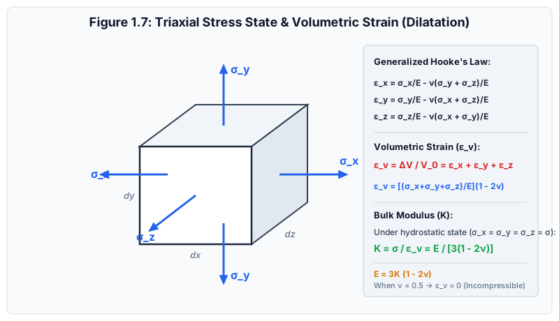
Consider a homogeneous, isotropic rectangular element subjected to triaxial normal stresses (σx,σy,σz\sigma_x, \sigma_y, \sigma_z) aligned with the principal Cartesian axes:

Triaxial Stress State and Volumetric Dilatation
Figure 1.7: Triaxial stress state acting on an infinitesimal 3D solid element illustrating volumetric dilatation and generalized Hooke's Law.

By the Principle of Superposition, the total normal strain in each direction is the sum of the direct strain produced by the stress in that direction plus the lateral Poisson contractions induced by the stresses in the other two orthogonal directions:

ϵx=σxE−νσyE−νσzE=1E[σx−ν(σy+σz)]ϵy=σyE−νσxE−νσzE=1E[σy−ν(σx+σz)]ϵz=σzE−νσxE−νσyE=1E[σz−ν(σx+σy)]\begin{aligned} \epsilon_x &= \frac{\sigma_x}{E} - \nu \frac{\sigma_y}{E} - \nu \frac{\sigma_z}{E} = \frac{1}{E} \left[ \sigma_x - \nu (\sigma_y + \sigma_z) \right] \\ \epsilon_y &= \frac{\sigma_y}{E} - \nu \frac{\sigma_x}{E} - \nu \frac{\sigma_z}{E} = \frac{1}{E} \left[ \sigma_y - \nu (\sigma_x + \sigma_z) \right] \\ \epsilon_z &= \frac{\sigma_z}{E} - \nu \frac{\sigma_x}{E} - \nu \frac{\sigma_y}{E} = \frac{1}{E} \left[ \sigma_z - \nu (\sigma_x + \sigma_y) \right] \end{aligned}

For pure shear stresses, isotropy implies uncoupling between normal stresses and shearing strains:

γxy=τxyG,γyz=τyzG,γzx=τzxG\gamma_{xy} = \frac{\tau_{xy}}{G}, \quad \gamma_{yz} = \frac{\tau_{yz}}{G}, \quad \gamma_{zx} = \frac{\tau_{zx}}{G}

3. Mathematical Derivations of the Interrelationships

3.1 Derivation of Volumetric Strain (ϵv\epsilon_v)

Consider a rectangular block of initial volume V0=LxLyLzV_0 = L_x L_y L_z. Under triaxial strains:

V=Lx(1+ϵx)⋅Ly(1+ϵy)⋅Lz(1+ϵz)=V0(1+ϵx)(1+ϵy)(1+ϵz)V = L_x(1 + \epsilon_x) \cdot L_y(1 + \epsilon_y) \cdot L_z(1 + \epsilon_z) = V_0 (1 + \epsilon_x)(1 + \epsilon_y)(1 + \epsilon_z)

Expanding and neglecting higher-order product terms of infinitesimal strains (ϵxϵy≈0\epsilon_x \epsilon_y \approx 0):

V≈V0(1+ϵx+ϵy+ϵz)V \approx V_0 (1 + \epsilon_x + \epsilon_y + \epsilon_z)

The change in volume is ΔV=V−V0=V0(ϵx+ϵy+ϵz)\Delta V = V - V_0 = V_0 (\epsilon_x + \epsilon_y + \epsilon_z). Therefore, the volumetric strain is:

ϵv=ΔVV0=ϵx+ϵy+ϵz\epsilon_v = \frac{\Delta V}{V_0} = \epsilon_x + \epsilon_y + \epsilon_z

Substituting Generalized Hooke's Law:

ϵv=1E[σx−ν(σy+σz)+σy−ν(σx+σz)+σz−ν(σx+σy)]=1E[(σx+σy+σz)−2ν(σx+σy+σz)]ϵv=σx+σy+σzE(1−2ν)\begin{aligned} \epsilon_v &= \frac{1}{E} \left[ \sigma_x - \nu(\sigma_y + \sigma_z) + \sigma_y - \nu(\sigma_x + \sigma_z) + \sigma_z - \nu(\sigma_x + \sigma_y) \right] \\ &= \frac{1}{E} \left[ (\sigma_x + \sigma_y + \sigma_z) - 2\nu(\sigma_x + \sigma_y + \sigma_z) \right] \\ \epsilon_v &= \frac{\sigma_x + \sigma_y + \sigma_z}{E} (1 - 2\nu) \end{aligned}

3.2 Derivation 1: Relationship between EE, KK, and ν\nu (E=3K(1−2ν)E = 3K(1 - 2\nu))

Consider a uniform hydrostatic stress field where all three normal stresses are equal:

σx=σy=σz=σ\sigma_x = \sigma_y = \sigma_z = \sigma

Substituting into the volumetric strain equation:

ϵv=σ+σ+σE(1−2ν)=3σE(1−2ν)\epsilon_v = \frac{\sigma + \sigma + \sigma}{E} (1 - 2\nu) = \frac{3\sigma}{E} (1 - 2\nu)

By definition of Bulk Modulus, K=σϵv  ⟹  ϵv=σKK = \frac{\sigma}{\epsilon_v} \implies \epsilon_v = \frac{\sigma}{K}. Equating the two expressions:

σK=3σE(1−2ν)\frac{\sigma}{K} = \frac{3\sigma}{E} (1 - 2\nu)

Canceling σ\sigma and rearranging yields the first core identity:

E=3K(1−2ν)E = 3K (1 - 2\nu)

3.3 Derivation 2: Relationship between EE, GG, and ν\nu (E=2G(1+ν)E = 2G(1 + \nu))

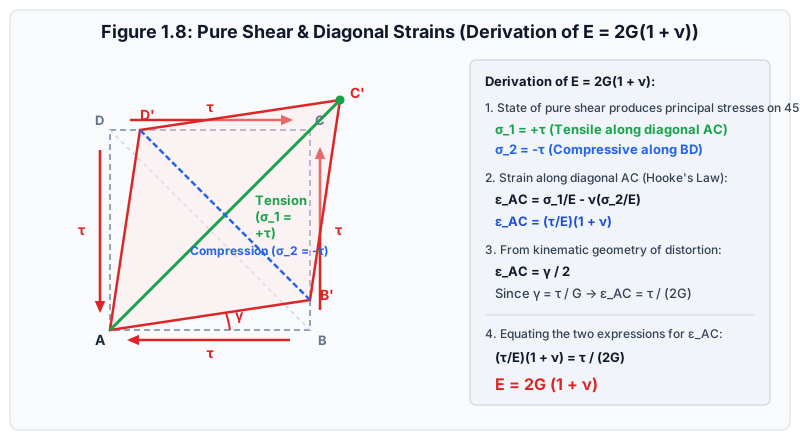
Consider an infinitesimal square element ABCDABCD of side length aa subjected to pure shear stress τ\tau:

Pure Shear and Diagonal Strains
Figure 1.8: Geometry of a square element under pure shear stress τ\tau, showing diagonal tensile elongation along AC and compressive contraction along BD.

Step 1: Principal Stresses on Diagonal Planes

A state of pure shear on mutually perpendicular planes is equivalent to equal and opposite principal normal stresses acting on planes inclined at 45∘45^\circ:

σ1=+τ(Tensile stress acting along diagonal AC)\sigma_1 = +\tau \quad (\text{Tensile stress acting along diagonal } AC) σ2=−τ(Compressive stress acting along diagonal BD)\sigma_2 = -\tau \quad (\text{Compressive stress acting along diagonal } BD)

Step 2: Linear Strain Along Diagonal ACAC from Hooke's Law

Applying Generalized Hooke's Law to the biaxial principal stress state (σ1=+τ,σ2=−τ\sigma_1 = +\tau, \sigma_2 = -\tau):

ϵAC=σ1E−νσ2E=τE−ν(−τE)=τE(1+ν)\epsilon_{AC} = \frac{\sigma_1}{E} - \nu \frac{\sigma_2}{E} = \frac{\tau}{E} - \nu \left(-\frac{\tau}{E}\right) = \frac{\tau}{E} (1 + \nu)

Step 3: Kinematic Strain Along Diagonal ACAC from Shear Distortion

Under shear stress τ\tau, the element deforms into a rhombus with shear strain γ=τ/G\gamma = \tau / G.
Let diagonal ACAC have initial length LAC=a2+a2=a2L_{AC} = \sqrt{a^2 + a^2} = a\sqrt{2}.
Due to small angular distortion γ\gamma, the change in length of diagonal ACAC is:

ΔLAC≈acos⁡45∘⋅γ=a22γ=a2γ\Delta L_{AC} \approx a \cos 45^\circ \cdot \gamma = a \frac{\sqrt{2}}{2} \gamma = \frac{a}{\sqrt{2}} \gamma

Therefore, the engineering strain along diagonal ACAC is:

ϵAC=ΔLACLAC=a2γa2=γ2\epsilon_{AC} = \frac{\Delta L_{AC}}{L_{AC}} = \frac{\frac{a}{\sqrt{2}} \gamma}{a \sqrt{2}} = \frac{\gamma}{2}

Since γ=τG\gamma = \frac{\tau}{G}:

ϵAC=τ2G\epsilon_{AC} = \frac{\tau}{2G}

Step 4: Equating Strains

Equating the Hookean strain to the kinematic strain:

τE(1+ν)=τ2G\frac{\tau}{E} (1 + \nu) = \frac{\tau}{2G}

Canceling τ\tau and solving for EE yields the second core identity:

E=2G(1+ν)E = 2G (1 + \nu)

3.4 Derivation 3: Master Formula Linking E,G,KE, G, K (E=9KG3K+GE = \frac{9KG}{3K + G})

From equation (1):

E=3K(1−2ν)  ⟹  1−2ν=E3K  ⟹  2ν=1−E3KE = 3K(1 - 2\nu) \implies 1 - 2\nu = \frac{E}{3K} \implies 2\nu = 1 - \frac{E}{3K}

From equation (2):

E=2G(1+ν)  ⟹  1+ν=E2G  ⟹  2ν=EG−2E = 2G(1 + \nu) \implies 1 + \nu = \frac{E}{2G} \implies 2\nu = \frac{E}{G} - 2

Equating the two expressions for 2ν2\nu:

1−E3K=EG−21 - \frac{E}{3K} = \frac{E}{G} - 2 3=EG+E3K=E(1G+13K)=E(3K+G3KG)3 = \frac{E}{G} + \frac{E}{3K} = E \left( \frac{1}{G} + \frac{1}{3K} \right) = E \left( \frac{3K + G}{3KG} \right)

Solving for EE:

E=9KG3K+GE = \frac{9KG}{3K + G}

3.5 Derivation 4: Poisson's Ratio in terms of KK and GG

Equating equation (1) and equation (2):

2G(1+ν)=3K(1−2ν)2G(1 + \nu) = 3K(1 - 2\nu) 2G+2Gν=3K−6Kν2G + 2G\nu = 3K - 6K\nu (6K+2G)ν=3K−2G(6K + 2G)\nu = 3K - 2G ν=3K−2G6K+2G\nu = \frac{3K - 2G}{6K + 2G}

4. Physical and Thermodynamic Bounds on Poisson's Ratio (ν\nu)

In classical continuum mechanics, the strain energy density function must be positive definite (an elastic body must always absorb positive mechanical work when strained):

  1. Condition 1 (G>0G > 0): E=2G(1+ν)>0  ⟹  1+ν>0  ⟹  ν>−1E = 2G(1 + \nu) > 0 \implies 1 + \nu > 0 \implies \nu > -1
  2. Condition 2 (K>0K > 0): E=3K(1−2ν)>0  ⟹  1−2ν>0  ⟹  ν<12=0.5E = 3K(1 - 2\nu) > 0 \implies 1 - 2\nu > 0 \implies \nu < \frac{1}{2} = 0.5

[!IMPORTANT] Fundamental Bounds:

  • Thermodynamic / Theoretical Limits (Isotropic): −1.0≤ν≤+0.5-1.0 \le \nu \le +0.5
  • Practical Engineering Solids: 0.0≤ν≤+0.50.0 \le \nu \le +0.5

4.1 Typical Poisson's Ratio Values for Civil Engineering Materials

Material Poisson's Ratio (ν\nu) Physical Behavior & Explanation
Cork ≈0.00\approx 0.00 Negligible lateral expansion under compression; ideal for bottle stoppers.
Structural Concrete 0.15−0.200.15 - 0.20 Moderate micro-cracking and void compression; IS 456 adopts ν=0.2\nu = 0.2 for uncracked sections.
Glass / Porous Rock 0.20−0.250.20 - 0.25 Brittle, highly rigid silicates with low lateral strain.
Cast Iron 0.23−0.270.23 - 0.27 Graphite flakes create low lateral expansion under axial load.
Structural Steel (Fe 250 / Fe 500) 0.28−0.300.28 - 0.30 Classic ductile metallic crystal lattice; IS 800 specifies ν=0.30\nu = 0.30.
Aluminum Alloys 0.330.33 Higher lateral contraction than steel.
Lead / Gold 0.42−0.450.42 - 0.45 Very soft, highly ductile metals.
Natural Rubber / Elastomers →0.50\to 0.50 (0.4990.499) Incompressible material: ϵv=0  ⟹  K→∞\epsilon_v = 0 \implies K \to \infty.
Saturated Clay (Undrained) ≈0.50\approx 0.50 Pore water carries pressure with zero instantaneous volume change.
Auxetic Materials / Polymer Foams <0< 0 (e.g. −0.7-0.7) Negative Poisson's ratio: expands laterally when stretched in tension!

5. Number of Independent Elastic Constants

The general linear Hooke's Law relating 6 stress components to 6 strain components contains 6×6=366 \times 6 = 36 stiffness coefficients in the compliance tensor. Thermodynamic conservation of strain energy reduces this to 21 independent coefficients for the most general, completely anisotropic material (triclinic crystal).

Symmetry conditions reduce the number of independent constants:

Material Symmetry Classification Total Elastic Constants Number of Independent Constants Examples
Anisotropic (General Triclinic) 36 21 Completely asymmetric rock, crystal structures
Orthotropic (Three mutually perpendicular planes of symmetry) 12 9 Timber, unidirectional fiber-reinforced composites
Transversely Isotropic (Rotational symmetry about one axis) 8 5 Layered soil strata, sedimentary rocks, rolled steel plates
Isotropic (Properties identical in all directions) 4 (E,G,K,νE, G, K, \nu) 2 Mild steel, aluminum, glass, brass

[!NOTE] For an isotropic material, knowing any two constants (e.g., EE and ν\nu, or KK and GG) uniquely determines the remaining two via the interrelationship equations.


6. Indian Standard (IS) Code Relevance

6.1 IS 456:2000 (Plain and Reinforced Concrete)

  • Clause 6.2.3.1: Poisson's ratio for concrete shall be taken as 0.200.20 for calculations involving uncracked structural elements, and may be taken as 0.00.0 when cracking is explicitly accounted for in design.
  • Clause 6.2.3.1: Modulus of elasticity of concrete: Ec=5000fck[MPa]E_c = 5000 \sqrt{f_{ck}} \quad [\text{MPa}]

6.2 IS 800:2007 (General Construction in Steel)

  • Table 1: Defines standard mechanical constants for structural steel design:
    • Modulus of Elasticity: E=2.0×10⁵ N/mm2E = 2.0 \times 10^5\text{ N/mm}^2
    • Modulus of Rigidity: G=0.769×10⁵ N/mm2≈0.77×105 N/mm2G = 0.769 \times 10^5\text{ N/mm}^2 \approx 0.77 \times 10^5\text{ N/mm}^2
    • Poisson's Ratio: ν=0.30\nu = 0.30
    • Coefficient of Thermal Expansion: α=12×10−6/∘C\alpha = 12 \times 10^{-6} / ^\circ\text{C}

7. Comparative Analysis Table

Characteristic Young's Modulus (EE) Shear Modulus (GG) Bulk Modulus (KK)
Type of Loading Uniaxial normal tension/compression Pure shear / torsion Uniform hydrostatic all-around pressure
Deformation Mode Linear longitudinal stretch/shortening Angular skewing / distortion (γ\gamma) Volumetric expansion/contraction (ΔV\Delta V)
Constant Volume? No (ΔV≠0\Delta V \ne 0) Yes (ΔV=0\Delta V = 0) No (ΔV≠0\Delta V \ne 0)
Typical Value (Steel) 200 GPa200\text{ GPa} ≈77 GPa\approx 77\text{ GPa} ≈160 GPa\approx 160\text{ GPa}
Relative Magnitude E>K>GE > K > G (for structural steel: 200>160>77200 > 160 > 77) Smallest of the moduli: G≈0.38EG \approx 0.38 E Intermediate: K≈0.83EK \approx 0.83 E

8. Step-by-Step Solved Numerical Examples

Example 3.1: Determination of KK and ν\nu from EE and GG (GATE CE Level)

Problem Statement:
An isotropic structural steel alloy coupon has a measured Young's modulus of E=200 GPaE = 200\text{ GPa} and a shear modulus of G=78 GPaG = 78\text{ GPa}. Calculate:

  1. Poisson's ratio (ν\nu) of the material.
  2. The bulk modulus (KK) of the material.
  3. Verify the master relationship E=9KG3K+GE = \frac{9KG}{3K + G}.

Step-by-Step Solution:

  1. Calculate Poisson's Ratio (ν\nu): Using E=2G(1+ν)E = 2G(1 + \nu):

    1+ν=E2G=200 GPa2×78 GPa=200156=1.2820511 + \nu = \frac{E}{2G} = \frac{200\text{ GPa}}{2 \times 78\text{ GPa}} = \frac{200}{156} = 1.282051 ν=1.282051−1=0.28205≈0.282\nu = 1.282051 - 1 = 0.28205 \approx 0.282
  2. Calculate Bulk Modulus (KK): Using E=3K(1−2ν)E = 3K(1 - 2\nu):

    1−2ν=1−2(0.282051)=1−0.564102=0.4358981 - 2\nu = 1 - 2(0.282051) = 1 - 0.564102 = 0.435898 K=E3(1−2ν)=200 GPa3×0.435898=2001.307694=152.9409 GPa≈152.94 GPaK = \frac{E}{3(1 - 2\nu)} = \frac{200\text{ GPa}}{3 \times 0.435898} = \frac{200}{1.307694} = 152.9409\text{ GPa} \approx 152.94\text{ GPa}
  3. Independent Verification Check: Compute EE using E=9KG3K+GE = \frac{9KG}{3K + G}:

    Numerator=9×152.9409×78=107,364.51\text{Numerator} = 9 \times 152.9409 \times 78 = 107,364.51 Denominator=3(152.9409)+78=458.8227+78=536.8227\text{Denominator} = 3(152.9409) + 78 = 458.8227 + 78 = 536.8227 E=107,364.51536.8227=200.000 GPa(Verified exact match)E = \frac{107,364.51}{536.8227} = 200.000\text{ GPa} \quad \text{(Verified exact match)}

Example 3.2: Triaxial Loading on a Rectangular Block (UPSC ESE Level)

Problem Statement:
A metallic prismatic block of dimensions 100 mm×80 mm×60 mm100\text{ mm} \times 80\text{ mm} \times 60\text{ mm} (along x,y,zx, y, z axes respectively) is subjected to the following triaxial normal stresses:

  • σx=+120 MPa\sigma_x = +120\text{ MPa} (Tension)
  • σy=−80 MPa\sigma_y = -80\text{ MPa} (Compression)
  • σz=+60 MPa\sigma_z = +60\text{ MPa} (Tension)

Given E=200 GPa=2×10⁵ N/mm2E = 200\text{ GPa} = 2 \times 10^5\text{ N/mm}^2 and Poisson's ratio ν=0.30\nu = 0.30.
Calculate:

  1. The linear strain along each principal axis (ϵx,ϵy,ϵz\epsilon_x, \epsilon_y, \epsilon_z).
  2. The volumetric strain (ϵv\epsilon_v).
  3. The absolute change in volume (ΔV\Delta V) of the block in mm3\text{mm}^3.

Step-by-Step Solution:

  1. Calculate Linear Strains: Using Generalized Hooke's Law:

    • For xx-direction (Lx=100 mmL_x = 100\text{ mm}):

      ϵx=1E[σx−ν(σy+σz)]=1200,000[120−0.30((−80)+60)]=1200,000[120−0.30(−20)]=1200,000[120+6]=126200,000=+6.30×10⁻⁴\begin{aligned} \epsilon_x &= \frac{1}{E} \left[ \sigma_x - \nu(\sigma_y + \sigma_z) \right] \\ &= \frac{1}{200,000} \left[ 120 - 0.30((-80) + 60) \right] \\ &= \frac{1}{200,000} \left[ 120 - 0.30(-20) \right] \\ &= \frac{1}{200,000} [ 120 + 6 ] = \frac{126}{200,000} = +6.30 \times 10^{-4} \end{aligned}
    • For yy-direction (Ly=80 mmL_y = 80\text{ mm}):

      ϵy=1E[σy−ν(σx+σz)]=1200,000[−80−0.30(120+60)]=1200,000[−80−0.30(180)]=1200,000[−80−54]=−134200,000=−6.70×10⁻⁴\begin{aligned} \epsilon_y &= \frac{1}{E} \left[ \sigma_y - \nu(\sigma_x + \sigma_z) \right] \\ &= \frac{1}{200,000} \left[ -80 - 0.30(120 + 60) \right] \\ &= \frac{1}{200,000} \left[ -80 - 0.30(180) \right] \\ &= \frac{1}{200,000} [ -80 - 54 ] = \frac{-134}{200,000} = -6.70 \times 10^{-4} \end{aligned}
    • For zz-direction (Lz=60 mmL_z = 60\text{ mm}):

      ϵz=1E[σz−ν(σx+σy)]=1200,000[60−0.30(120+(−80))]=1200,000[60−0.30(40)]=1200,000[60−12]=48200,000=+2.40×10⁻⁴\begin{aligned} \epsilon_z &= \frac{1}{E} \left[ \sigma_z - \nu(\sigma_x + \sigma_y) \right] \\ &= \frac{1}{200,000} \left[ 60 - 0.30(120 + (-80)) \right] \\ &= \frac{1}{200,000} \left[ 60 - 0.30(40) \right] \\ &= \frac{1}{200,000} [ 60 - 12 ] = \frac{48}{200,000} = +2.40 \times 10^{-4} \end{aligned}
  2. Calculate Volumetric Strain (ϵv\epsilon_v):

    • Method A (Sum of Strains): ϵv=ϵx+ϵy+ϵz=(6.30−6.70+2.40)×10−4=+2.00×10⁻⁴\epsilon_v = \epsilon_x + \epsilon_y + \epsilon_z = (6.30 - 6.70 + 2.40) \times 10^{-4} = +2.00 \times 10^{-4}
    • Method B (Analytical Formula Check): ϵv=σx+σy+σzE(1−2ν)\epsilon_v = \frac{\sigma_x + \sigma_y + \sigma_z}{E} (1 - 2\nu) σx+σy+σz=120−80+60=100 MPa\sigma_x + \sigma_y + \sigma_z = 120 - 80 + 60 = 100\text{ MPa} 1−2ν=1−2(0.30)=0.401 - 2\nu = 1 - 2(0.30) = 0.40 ϵv=100200,000×0.40=(5.0×10−4)×0.40=+2.00×10⁻⁴(Verified exact)\epsilon_v = \frac{100}{200,000} \times 0.40 = (5.0 \times 10^{-4}) \times 0.40 = +2.00 \times 10^{-4} \quad \text{(Verified exact)}
  3. Calculate Change in Volume (ΔV\Delta V): Initial Volume:

    V0=100 mm×80 mm×60 mm=480,000 mm3V_0 = 100\text{ mm} \times 80\text{ mm} \times 60\text{ mm} = 480,000\text{ mm}^3

    Change in Volume:

    ΔV=ϵv×V0=(2.00×10−4)×480,000 mm3=+96.0 mm3\Delta V = \epsilon_v \times V_0 = (2.00 \times 10^{-4}) \times 480,000\text{ mm}^3 = +96.0\text{ mm}^3

    Conclusion: The block expands in volume by 96 mm396\text{ mm}^3.


Example 3.3: Incompressible Elastomer Under Rigid Lateral Constraint (SSC JE / State AE Level)

Problem Statement:
A rubber cylinder of diameter d=50 mmd = 50\text{ mm} and length L=100 mmL = 100\text{ mm} with Poisson's ratio ν=0.50\nu = 0.50 is fitted snugly inside a completely rigid steel cylinder (preventing any lateral radial expansion). An axial compressive load of P=20 kNP = 20\text{ kN} is applied to the rubber cylinder.
Determine:

  1. The lateral compressive stress (σr\sigma_r) induced on the walls of the rigid cylinder.
  2. The axial deformation (ΔL\Delta L) of the rubber cylinder if E=10 MPaE = 10\text{ MPa}.

Step-by-Step Solution:

  1. Boundary Conditions:

    • Lateral radial expansion is completely prevented: ϵr=ϵy=ϵz=0\epsilon_r = \epsilon_y = \epsilon_z = 0.
    • Lateral stresses induced symmetrically: σy=σz=σr\sigma_y = \sigma_z = \sigma_r.
    • Axial stress: σx=−PA\sigma_x = - \frac{P}{A}. A=π4(50 mm)2=625π mm2≈1963.4954 mm2A = \frac{\pi}{4} (50\text{ mm})^2 = 625 \pi\text{ mm}^2 \approx 1963.4954\text{ mm}^2 σx=−20,000 N1963.4954 mm2=−10.1859 MPa\sigma_x = -\frac{20,000\text{ N}}{1963.4954\text{ mm}^2} = -10.1859\text{ MPa}
  2. Lateral Stress Induced (σr\sigma_r): Applying Hooke's Law for lateral strain:

    ϵr=σrE−νσx+σrE=0\epsilon_r = \frac{\sigma_r}{E} - \nu \frac{\sigma_x + \sigma_r}{E} = 0 σr−νσx−νσr=0  ⟹  σr(1−ν)=νσx\sigma_r - \nu \sigma_x - \nu \sigma_r = 0 \implies \sigma_r (1 - \nu) = \nu \sigma_x σr=(ν1−ν)σx\sigma_r = \left(\frac{\nu}{1 - \nu}\right) \sigma_x

    Since the rubber is incompressible (ν=0.50\nu = 0.50):

    ν1−ν=0.501−0.50=0.500.50=1.0\frac{\nu}{1 - \nu} = \frac{0.50}{1 - 0.50} = \frac{0.50}{0.50} = 1.0

    Therefore:

    σr=1.0×σx=−10.1859 MPa≈−10.19 MPa\sigma_r = 1.0 \times \sigma_x = -10.1859\text{ MPa} \approx -10.19\text{ MPa}

    Physical Meaning: An incompressible solid with ν=0.50\nu = 0.50 under complete lateral constraint acts like an ideal hydraulic fluid, transmitting 100%100\% of the axial pressure laterally to the container walls (σr=σx\sigma_r = \sigma_x).

  3. Axial Strain and Deformation (ΔL\Delta L):

    ϵx=σxE−νσr+σrE=1E[σx−2νσr]\epsilon_x = \frac{\sigma_x}{E} - \nu \frac{\sigma_r + \sigma_r}{E} = \frac{1}{E} \left[ \sigma_x - 2\nu \sigma_r \right]

    Since ν=0.50\nu = 0.50 and σr=σx\sigma_r = \sigma_x:

    ϵx=1E[σx−2(0.50)σx]=1E[σx−σx]=0!\epsilon_x = \frac{1}{E} \left[ \sigma_x - 2(0.50)\sigma_x \right] = \frac{1}{E} [ \sigma_x - \sigma_x ] = 0 ! ΔL=ϵx×L=0.0 mm\Delta L = \epsilon_x \times L = 0.0\text{ mm}

Physical Verification Check:
Because the material is incompressible (ϵv=0\epsilon_v = 0) and its lateral boundary is completely rigid (ϵlateral=0\epsilon_{\text{lateral}} = 0), it cannot deform axially either (ϵaxial=ϵv−2ϵlateral=0−0=0\epsilon_{\text{axial}} = \epsilon_v - 2\epsilon_{\text{lateral}} = 0 - 0 = 0). The rubber exhibits infinite apparent compressive stiffness under full volumetric confinement!


9. Common Pitfalls & Competitive Exam Traps

[!WARNING] Trap 1: The Minus Sign in Poisson's Ratio Definition
Students often forget whether Poisson's ratio is positive or negative.
By definition, ν=−ϵlatϵlong\nu = -\frac{\epsilon_{\text{lat}}}{\epsilon_{\text{long}}}. For normal materials, ϵlat\epsilon_{\text{lat}} is opposite in sign to ϵlong\epsilon_{\text{long}}, so ν\nu is a positive number (0.25−0.300.25 - 0.30). Only rare synthetic auxetic materials have negative Poisson's ratios.

[!WARNING] Trap 2: The Ratio G/EG/E and K/EK/E Limits
For engineering materials (0≤ν≤0.50 \le \nu \le 0.5):

  • Since E=2G(1+ν)E = 2G(1+\nu):
    • At ν=0  ⟹  G=0.50E  ⟹  G/E=0.50\nu = 0 \implies G = 0.50 E \implies G/E = 0.50 (Maximum)
    • At ν=0.5  ⟹  G=E3≈0.333E  ⟹  G/E=0.333\nu = 0.5 \implies G = \frac{E}{3} \approx 0.333 E \implies G/E = 0.333 (Minimum)
    • Thus: 13≤GE≤12\frac{1}{3} \le \frac{G}{E} \le \frac{1}{2}
  • Since E=3K(1−2ν)E = 3K(1-2\nu):
    • At ν=0  ⟹  K=E3  ⟹  K/E=0.333\nu = 0 \implies K = \frac{E}{3} \implies K/E = 0.333 (Minimum)
    • At ν=0.5  ⟹  K→∞  ⟹  K/E→∞\nu = 0.5 \implies K \to \infty \implies K/E \to \infty (Maximum)
    • Thus: KE≥13\frac{K}{E} \ge \frac{1}{3} These ratio limits are tested frequently in GATE Multiple Select Questions (MSQ).

[!WARNING] Trap 3: Number of Independent Constants in Anisotropic Materials
Many students confuse the total number of tensor elements (3636) with the number of independent elastic constants (2121). Always remember:

  • General Anisotropic = 21
  • Orthotropic = 9
  • Isotropic = 2

10. Quick Revision Formula Box

Relation 1:E=2G(1+ν)Relation 2:E=3K(1−2ν)Relation 3 (Master):E=9KG3K+GRelation 4 (Poisson):ν=3K−2G6K+2GVolumetric Strain:ϵv=ϵx+ϵy+ϵz=σx+σy+σzE(1−2ν)Hydrostatic Volumetric Strain:ϵv=3σE(1−2ν)=σKThermodynamic Bounds:−1.0≤ν≤+0.50Engineering Bounds:0.0≤ν≤+0.50Incompressible Solid:ν=0.50  ⟹  ϵv=0,K→∞\begin{aligned} \text{Relation 1:} \quad E &= 2G(1 + \nu) \\ \text{Relation 2:} \quad E &= 3K(1 - 2\nu) \\ \text{Relation 3 (Master):} \quad E &= \frac{9KG}{3K + G} \\ \text{Relation 4 (Poisson):} \quad \nu &= \frac{3K - 2G}{6K + 2G} \\ \text{Volumetric Strain:} \quad \epsilon_v &= \epsilon_x + \epsilon_y + \epsilon_z = \frac{\sigma_x + \sigma_y + \sigma_z}{E}(1 - 2\nu) \\ \text{Hydrostatic Volumetric Strain:} \quad \epsilon_v &= \frac{3\sigma}{E}(1 - 2\nu) = \frac{\sigma}{K} \\ \text{Thermodynamic Bounds:} \quad -1.0 &\le \nu \le +0.50 \\ \text{Engineering Bounds:} \quad 0.0 &\le \nu \le +0.50 \\ \text{Incompressible Solid:} \quad \nu &= 0.50 \implies \epsilon_v = 0, \quad K \to \infty \end{aligned}

11. References & Source Literature

  1. Timoshenko, S. P., & Goodier, J. N. (1970). Theory of Elasticity, 3rd Edition, McGraw-Hill, New York.
  2. Gere, J. M., & Goodno, B. J. (2018). Mechanics of Materials, 9th Edition, Cengage Learning, Boston.
  3. Punmia, B. C., Jain, A. K., & Jain, A. K. (2017). Mechanics of Materials, 15th Edition, Laxmi Publications, New Delhi.
  4. Bureau of Indian Standards (2000). IS 456:2000 — Plain and Reinforced Concrete - Code of Practice, New Delhi.
  5. Bureau of Indian Standards (2007). IS 800:2007 — General Construction in Steel - Code of Practice, New Delhi.