Strain Energy & Castigliano's Theorem for Beam Deflections
In this chapter (4 topics)
On this page
- 1. Engineering Context & Overview
- 2. Internal Work & Strain Energy in Pure Bending
- 2.1 Axial and Shear Energy Contributions
- 3. Castigliano's Theorems (First & Second)
- 3.1 Strain Energy (U) vs Complementary Strain Energy (U*)
- 3.2 Castigliano's First Theorem
- 3.3 Castigliano's Second Theorem
- 4. Leibniz's Rule: Differentiation Under the Integral Sign
- Practical Advantage of Differentiating Under the Integral Sign
- 5. The Fictitious (Dummy) Load Method & Virtual Work Equivalence
- 5.1 The Problem of Unloaded Points
- 5.2 Equivalence to the Unit Load Method (Principle of Virtual Work)
- 6. Deflections of Bent Cantilevers, Frames & Curved Members
- 6.1 Orthogonal Bent Frames (L-Shaped Cantilever)
- 6.2 Curved Beams and Rings in Their Plane
- 7. Engineering Diagrams & Visual Walkthrough
- Figure 1: Castigliano's Theorems & Flexural Strain Energy
- Figure 2: Dummy Load Method & Curved Beam Deflection
- 8. Worked Numerical Examples
- Example 1: Cantilever with Combined Full UDL and Tip Load
- Example 2: Orthogonal L-Frame Bent Cantilever
- Example 3: Quarter-Circular Cantilever Curved Bar
- 9. Comprehensive Beam Deflection Method Selection Matrix
- 10. Common Misconceptions & Exam Pitfalls
- 11. Real-World Engineering Applications & Standard Codes
- 12. Quick Revision Summary & Formula Sheet
1. Engineering Context & Overview
While geometric methods (Double Integration, Macaulay's Method, Moment-Area, and Conjugate Beam) rely directly on the differential relationship between curvature and bending moment (), energy methods operate on the fundamental principle of Conservation of Energy.
For structures undergoing non-uniform flexure, internal strain energy () is stored in the elastic material fibers. Alberto Castigliano (1847–1884) demonstrated that partial derivatives of this internal energy with respect to external generalized loads yield the corresponding generalized displacements directly.
In modern structural engineering and competitive examinations (GATE CE, UPSC ESE), Castigliano's Second Theorem and its corollary, the Dummy (Fictitious) Load Method, serve as the most potent tools for solving:
- Complex non-prismatic members and bent cantilevers (orthogonal frames).
- Deflections and rotations in curved beams, arches, and circular rings where classical geometric curvature integration becomes analytically prohibitive.
- Statically indeterminate beams where internal redundant reactions can be solved by setting the partial derivative of strain energy with respect to the redundant force to zero (Principle of Least Work).
2. Internal Work & Strain Energy in Pure Bending
Consider an elastic beam subject to transverse loading. At any cross-section at distance , an internal bending moment acts. Over an infinitesimal element of length , the relative angular rotation of the two opposite transverse faces is given by:
Under gradually applied static loads within the proportional limit (), the relationship between bending moment and relative rotation is strictly linear. The incremental internal strain energy stored in this infinitesimal segment is the area under the linear diagram:
Integrating over the entire beam length (or summing over all distinct structural segments):
   Face A           Element dx           Face B
     │                                     │
     │◄─────────────── dx ───────────────►│
     │                                     │
 ───┼─────────────────────────────────────┼─── Neutral Axis
     │                                     │
     ▼ M(x) (Sagging)                      ▲ M(x) + dM
    (                                     )
    Rel. Rotation dθ = [M(x) / EI] dx
    Incremental Strain Energy: dU = ½ M(x) dθ = [M(x)² / (2EI)] dx
2.1 Axial and Shear Energy Contributions
In general structural members, strain energy is also produced by axial force , shear force , and torque :
where is the shear form factor ( for rectangular sections, for circular sections).
Important Engineering Observation: For slender beams where the span-to-depth ratio exceeds 10 (), flexural strain energy accounts for more than 98% to 99% of the total stored internal energy. Consequently, in all standard competitive examinations (GATE CE, ESE), shear and axial strain energy contributions in beam deflection are routinely neglected unless shear deformation is explicitly requested (Timoshenko beam theory).
3. Castigliano's Theorems (First & Second)
3.1 Strain Energy () vs Complementary Strain Energy ()
For an elastic body loaded by generalized forces resulting in generalized displacements :
- Internal Strain Energy (): Stored as internal fiber strain:
- Complementary Strain Energy (): Mathematical dual defined with respect to force increments:
For non-linear elastic materials, . However, for linearly elastic materials obeying Hooke's Law, the force-displacement diagram is a straight line through the origin, making:
3.2 Castigliano's First Theorem
Statement: In any elastic system at constant temperature, the first partial derivative of the total internal strain energy () with respect to any generalized displacement () equals the corresponding generalized external force () acting at that point in the direction of .
Scope: Valid for both linear and non-linear elastic structures. Primarily utilized in displacement-based finite element formulations and stiffness matrix derivations.
3.3 Castigliano's Second Theorem
Statement: In any linearly elastic structure at constant temperature with unyielding supports, the first partial derivative of the total internal strain energy () with respect to any generalized external force () equals the generalized displacement () at the point of application of along its line of action.
Similarly for rotations: If an external moment / couple acts at a node, the rotation at that point in the direction of is:
Scope: Strictly restricted to linearly elastic systems (Hooke's Law valid, principle of superposition holds, ).
4. Leibniz's Rule: Differentiation Under the Integral Sign
Directly substituting and attempting to square the algebraic moment expressions before integrating leads to severe algebraic expansion errors.
By invoking Leibniz's Integral Rule, we differentiate with respect to inside the integral sign:
Similarly, the rotation at point is:
Practical Advantage of Differentiating Under the Integral Sign
- Reduces Polynomial Degree: Instead of integrating (which could be degree 4 or 6 for UDL/varying loads), we integrate the product of and its linear partial derivative .
- Allows Setting Fictitious Loads to Zero Before Integration: As shown in Section 5, if is a fictitious dummy load, it can be set to zero prior to computing the integral, vastly simplifying the algebra.
5. The Fictitious (Dummy) Load Method & Virtual Work Equivalence
5.1 The Problem of Unloaded Points
Castigliano's Second Theorem requires an active external concentrated force (or moment) at the exact point and in the exact direction of the desired deflection (or rotation). If the desired displacement occurs at a point where no load acts (or where only a distributed load acts):
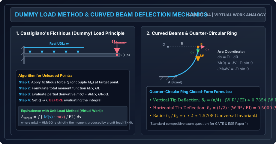
- Step 1 (Introduce Fictitious Load): Apply an imaginary fictitious concentrated force (or fictitious moment ) at the point of interest in the assumed direction of displacement.
- Step 2 (Formulate Moment Equation): Write the section bending moment expression as a function of real loads and the fictitious parameter: .
- Step 3 (Differentiate Partially): Evaluate the partial derivative with respect to :
- Step 4 (Set Dummy Load to Zero): Evaluate the limit as inside the integral:
5.2 Equivalence to the Unit Load Method (Principle of Virtual Work)
Notice that:
represents the internal bending moment produced throughout the structure when a single concentrated load of unit magnitude () is applied at the desired displacement location!
Thus, Castigliano's fictitious load formulation is mathematically identical to the classic Unit Load Method (Dummy Unit Load):
where:
- = Bending moment due to actual applied loads.
- = Bending moment due to a fictitious unit load ( or ) applied at the target point.
6. Deflections of Bent Cantilevers, Frames & Curved Members
Energy methods excel where classical Cartesian coordinates break down.
6.1 Orthogonal Bent Frames (L-Shaped Cantilever)
For an L-frame fixed at base , with vertical column (height ) and horizontal cantilever beam (length ):
The displacements at tip are obtained by integrating over both orthogonal segments independently.
6.2 Curved Beams and Rings in Their Plane
For a curved beam of centroidal radius , an arc element has length . Neglecting axial and shear contributions for slender rings ():
For a quarter-circular cantilever ring of radius fixed at (vertical tangent) and free at , subjected to a vertical downward load :
- Coordinate measured from free end: .
- Moment at angle : .
- Derivative with respect to : .
- Vertical deflection:
- Horizontal deflection (via dummy horizontal force ):
- Universal Ratio:
7. Engineering Diagrams & Visual Walkthrough
Figure 1: Castigliano's Theorems & Flexural Strain Energy
The following diagram illustrates the relationship between strain energy and complementary strain energy , the physical flexure of an infinitesimal beam element, and Leibniz's rule for direct differentiation.
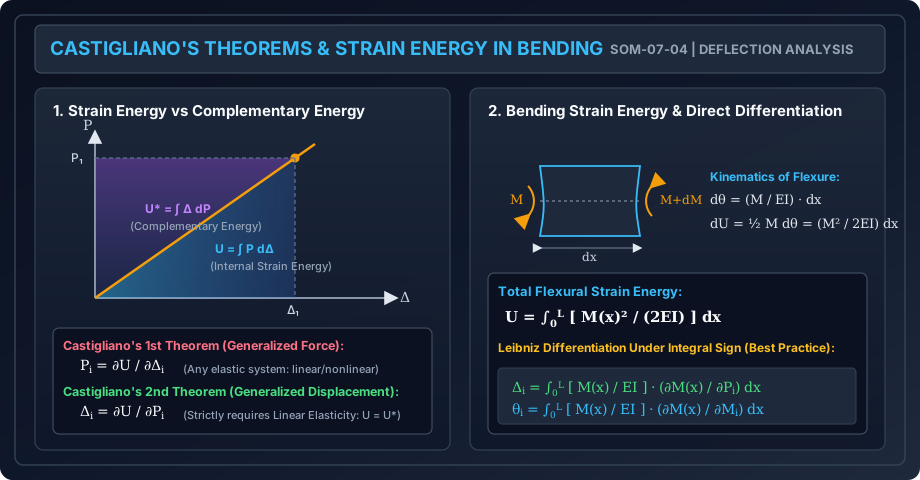
Figure 2: Dummy Load Method & Curved Beam Deflection
The following diagram demonstrates the 4-step algorithm for applying fictitious loads to unloaded points, its equivalence to the virtual unit load method, and closed-form deflection kinematics for curved rings.
8. Worked Numerical Examples
Example 1: Cantilever with Combined Full UDL and Tip Load
Problem Statement: A cantilever beam of span is fixed at and free at . It carries a uniformly distributed load over its entire length and a concentrated vertical downward load at the free tip .
Given flexural rigidity (, ).
Using Castigliano's Second Theorem:
- Determine the vertical downward deflection at tip .
- Determine the rotation (slope) at tip using the fictitious couple technique.
       w = 12 kN/m
  ══════════════════════════▼ P = 20 kN
  │█████████████████████████│
  │A                       B│
  │◄──────── 3.0 m ────────►│
  Fixed                   Free
Solution:
Part 1: Vertical Deflection
Let origin be at the free tip , with coordinate measured towards the fixed support ().
At any section :
Since acts directly at in the direction of the desired deflection, differentiate partially with respect to :
Applying Castigliano's Theorem:
Substitute the numerical parameters:
- Total numerator
Part 2: Slope (Rotation) at Tip
There is no concentrated moment acting at tip . Therefore, apply a fictitious clockwise couple at tip .
The bending moment at section becomes:
Differentiate partially with respect to :
Now set and integrate:
Substitute the parameters:
- Total numerator
Example 2: Orthogonal L-Frame Bent Cantilever
Problem Statement: An L-shaped rigid frame consists of a vertical member of height fixed at base , and a horizontal member of length rigidly joined at at knee . At the free tip , two concurrent concentrated loads act: a vertical downward load and a horizontal load directed towards the right.
Both members have identical flexural rigidity . Neglecting axial and shear deformation, calculate:
- The vertical deflection at .
- The horizontal deflection at .
           B ═════════════════════════ C ──► Q = 10 kN
           ║                           │
           ║                           ▼ P = 15 kN
    H = 2m ║
           ║
         ══╩══ A (Fixed Base)
           ◄──────── L = 3m ──────────►
Solution:
We break the structure into two segments: and .
1. Member (Horizontal leg, length ):
Let origin be at free end , with coordinate directed towards ():
Notice that the horizontal force acts axially along and induces zero bending moment in .
2. Member (Vertical leg, height ):
Let origin be at knee , with coordinate directed downwards towards base ().
The vertical force acts at lever arm , producing a constant hogging moment .
The horizontal force acts at lever arm from knee , producing an additional bending moment :
Vertical Deflection at :
Substitute the numerical values:
- Total numerator
Horizontal Deflection at :
Since , member contributes zero flexural displacement to :
Substitute the numerical values:
- Total numerator
Example 3: Quarter-Circular Cantilever Curved Bar
Problem Statement: A slender curved bar in the form of a quarter of a circle of radius lies in a vertical plane. The lower end is rigidly built-in (tangent is vertical), while the upper end is free (tangent is horizontal). A vertical concentrated downward load is applied at free end .
Given flexural rigidity . Neglecting axial and shear strains:
- Calculate the vertical downward deflection at .
- Calculate the horizontal deflection at .
- Verify the ratio .
Solution:
Let angular coordinate be measured from the free tip ():
- Arc differential length: .
- At section , the horizontal distance from to the section is .
- Therefore, the bending moment due to is:
- To obtain the horizontal deflection, apply a fictitious horizontal load directed to the right at tip . The vertical distance from down to the section is .
- The total moment including the dummy load is:
Taking partial derivatives:
1. Vertical Deflection :
Since :
Substitute the values (, , ):
2. Horizontal Deflection : Set in the integrand:
Evaluating the definite integral:
Integral value .
3. Ratio Verification:
The analytical prediction is perfectly verified.
9. Comprehensive Beam Deflection Method Selection Matrix
With all four deflection methods now mastered across Chapter 07, civil engineers must select the optimal method based on structural configuration:
| Method | Best Suited For | Critical Limitations | Exam Preference |
|---|---|---|---|
| Double Integration | Uniform, single-segment prismatic beams () with continuous loading. | Cumbersome for multiple point loads and discontinuous spans due to boundary constants. | Textbooks & basic derivations; rarely used in GATE for complex beams. |
| Macaulay's Method | Prismatic simply supported beams with multiple concentrated loads and partial UDLs. | Not suited for stepped/variable cross-sections () or curved geometries. | Highest priority for SSC JE, State AE, and standard GATE prismatic beams. |
| Moment-Area (Mohr) | Stepped / non-prismatic cantilevers, symmetric spans, and locations of known zero slope. | Difficult when neither slope nor tangent point is readily known (e.g., unsymmetric beams). | Best for stepped cantilevers and fixed-end moment derivations. |
| Conjugate Beam | Complex support configurations, internal hinges, overhanging spans, non-prismatic sections. | Requires converting supports; sign conventions of conjugate shear/moment can trip students. | Standard method for GATE / ESE involving internal hinges and overhangs. |
| Castigliano / Strain Energy | Orthogonal bent frames, portal frames, trusses, and curved rings / circular arches. | Computationally tedious for long multi-span continuous beams; requires dummy loads for unloaded points. | Mandatory method for curved members, frames, and indeterminate reactions. |
10. Common Misconceptions & Exam Pitfalls
[!WARNING] Pitfall 1: Squaring the Moment Expression Before Differentiating Expanding before taking the derivative leads to massive polynomial terms and inevitable algebraic errors. Always differentiate under the integral sign first: .
[!CAUTION] Pitfall 2: Forgetting to Set the Dummy Load to Zero Before Integration Students often keep as a variable throughout the integration, resulting in pages of wasted algebra. Once the partial derivative has been computed, set immediately inside the integrand before computing the integral.
[!WARNING] Pitfall 3: Applying Castigliano's 2nd Theorem to Non-Linear Elastic Systems Castigliano's Second Theorem () is derived from the equality of strain energy and complementary energy (). It is strictly valid only for linear elastic materials. For non-linear elastic systems, ; instead, Engesser's theorem applies: .
[!NOTE] Pitfall 4: Neglecting Member Contributions in Bent Frames In bent cantilevers (such as the L-frame in Example 2), students frequently evaluate the integral only for the member carrying the direct load (), completely forgetting that the vertical leg () undergoes flexure from the transferred moment and contributes significantly to both vertical and horizontal tip displacements.
11. Real-World Engineering Applications & Standard Codes
- Deflection Limits in IS 456:2000 (Clause 23.2):
- The final deflection due to all loads including the effects of temperature, creep, and shrinkage should not normally exceed .
- Deflection including effects of temperature, creep, and shrinkage occurring after erection of partitions and application of finishes should not exceed or , whichever is less.
- Deflection Limits in IS 800:2007 (Table 6):
- Industrial building crane gantry girders: (electric overhead travelling crane) or (manually operated).
- Roof purlins and building rafters: (elastic sheet roofing) or (brittle tile roofing).
- Curved Structural Elements:
- Circular arch ribs, tunnel linings, and expansion loops in high-pressure steam and oil piping rely directly on Castigliano's strain energy formulations to absorb thermal expansion displacements without exceeding permissible flexural stresses.
12. Quick Revision Summary & Formula Sheet
| Physical Quantity / Condition | Formula / Expression | Units |
|---|---|---|
| Bending Strain Energy () | or | |
| Castigliano's 1st Theorem | or | |
| Castigliano's 2nd Theorem (Displacement) | or | |
| Castigliano's 2nd Theorem (Rotation) | ||
| Dummy / Unit Load Method | or | |
| Quarter-Circular Ring (Vertical Tip Deflection) | or | |
| Quarter-Circular Ring (Horizontal Tip Deflection) | or | |
| Universal Ring Deflection Ratio | Dimensionless | |
| L-Frame Vertical Deflection (Tip Load ) | or |