Drag and Lift Forces on Submerged Bodies, Bluff vs Streamlined Bodies, Kármán Vortex Street & Magnus Effect
In this chapter (3 topics)
On this page
- 1. Module Overview & Pedagogical Scope
- 2. Official Examination Syllabus Mapping
- 3. Fundamental Physical Principles & Governing Assumptions
- 4. Mathematical Derivations & Rigorous Proofs
- Sub-derivation A: General Hydrodynamic Force Decomposition
- Sub-derivation B: Creeping Flow Past a Sphere & Stokes' Law (Re < 0.2)
- Sub-derivation C: The Drag Crisis (Eiffel Paradox) on Cylinders & Spheres
- Sub-derivation D: Von Kármán Vortex Street Hydrodynamics & Vortex-Induced Vibration
- Sub-derivation E: Kutta-Joukowski Lift Theorem & The Magnus Effect
- 5. Technical Diagrams & Interactive Architectural Schematics
- Figure 1: Total Hydrodynamic Drag Decomposition & Bluff vs Streamlined Spectrum
- Figure 2: Von Kármán Vortex Street Dynamics & Magnus Rotor Propulsion
- 6. Comparative Engineering Analysis & Parameter Regimes
- 7. Worked Numerical Examples (Pre-Calculated & Verified)
- Problem 1: Industrial Chimney Subjected to Hurricane Winds & Vortex Shedding
- Problem 2: Silt Settling in Water vs Parachute Descent Terminal Velocity
- Problem 3: Flettner Rotor Cargo Ship & The Magnus Effect
- 8. High-Yield Examination Traps & Ambiguities
- 9. Real-World Engineering Applications & Case Studies
- 10. Cross-Disciplinary & Downstream Dependencies
- 11. Summary Formula Cheat Sheet & Memory Anchors
- 12. Comprehensive References & Standard Codes
1. Module Overview & Pedagogical Scope
When a solid body is completely submerged in a moving fluid stream (or moves through a stationary fluid), the relative motion generates sustained normal pressure distributions and tangential wall shear stresses over its entire wetted surface. The vector integration of these surface stresses yields a net resultant hydrodynamic force .
In classical aerodynamics and fluid dynamics, this force is resolved into two mutually perpendicular components with respect to the undisturbed free-stream approach velocity vector :
- Drag Force (): The force component acting strictly parallel to the direction of relative approach velocity . Drag represents the total mechanical resistance opposing the relative motion.
- Lift Force (): The force component acting strictly perpendicular to the undisturbed approach velocity .
                      Resultant Force Resolution
                               FL (Lift)
                                  ▲
                                  │   / FR (Resultant)
                                  │  /
                                  │ /  θ
               Approach Flow ─────┼─────────► FD (Drag)
                    U∞            │
This master technical module establishes the comprehensive mechanics of fluid-structure interaction for external submerged flows across the complete spectrum from pure skin-friction dominated geometries (thin flat plates parallel to the stream) to severe pressure-drag dominated bluff bodies (flat plates normal to flow, circular cylinders, spheres, chimneys, bridge decks, and structural pylons).
We explore the exact analytical solution for low-Reynolds creeping flow (Stokes' law), the hydrodynamic physics governing the abrupt "Drag Crisis" (Eiffel paradox), the periodic shedding dynamics of the Von Kármán vortex street with associated vortex-induced vibrations (VIV) and lock-in, and the generation of asymmetrical circulation lift via the Kutta-Joukowski theorem and the Magnus effect on rotating bodies.
2. Official Examination Syllabus Mapping
Website note: this mapping is from the author’s notes. It has not been checked against the official notification for each examination; confirm the current syllabus with the examining body.
| Examination Body | Syllabus Code & Topics | Core Weightage & Target Focus |
|---|---|---|
| GATE (Civil Engineering) | Water Resources: Fluid Mechanics — Drag and lift forces on immersed bodies; Total drag decomposition into skin friction and pressure drag; Bluff and streamlined bodies; Separation around cylinders and spheres; Drag crisis; Vortex shedding and Strouhal number; Magnus effect. | High (1 to 2 questions yearly): Calculation of drag force, terminal settling velocities, vortex shedding frequencies, and lift-to-drag ratios. |
| UPSC ESE (Prelims & Mains) | Paper-II: Fluid Mechanics — External flows, pressure drag vs friction drag, flow past circular cylinders and spheres, circulation and lift, Kutta-Joukowski theorem, Magnus effect, aerodynamic streamlining of structural elements. | Very High: Analytical derivations of Stokes' law, drag crisis physics, VIV mitigation in chimneys, and multi-part numerical problems. |
| SSC JE & RRB JE | Civil Engineering / Fluid Mechanics — Terminal velocity of particles, definition of drag and lift coefficients, bluff vs streamlined shapes, causes of vortex shedding. | Direct / Objective: Formulae for , Stokes settling velocity , Strouhal number definition. |
| State AE / JE (All States) | Fluid Mechanics — Boundary layer separation impact on drag, terminal velocity in sediment basins, Magnus effect applications, wind loads on tall structures (IS 875 Part 3). | Objective & Numerical: Settling velocity of sediment, wind forces on poles, drag coefficient transitions. |
3. Fundamental Physical Principles & Governing Assumptions
- Continuum Hypothesis: The fluid medium is treated as a continuous, isotropic Newtonian fluid governed by constant dynamic viscosity and density .
- Coordinate Orientation: The undisturbed free-stream approach velocity vector is aligned with the positive -axis.
- Stress Decomposition: At any local differential surface area element with outward unit normal vector :
- The thermodynamic static pressure acts normal to the surface in the inward direction ().
- The viscous wall shear stress acts tangentially to the surface in the direction of local boundary shear.
- Projected Area Convention:
- For bluff bodies (cylinders, spheres, vehicles, structural members), the reference area in drag calculations is traditionally the frontal projected area normal to the flow: .
- For streamlined bodies (airfoils, hydrofoils, thin flat plates), the reference area is typically the planform area (chord span) or total wetted surface area.
- Incompressible Flow Assumption: Mach number , ensuring spatial invariance of fluid density .
- Separation-Induced Wake Deficit: In bluff body flows, boundary layer separation creates a wide, turbulent low-pressure wake zone downstream. The pressure difference between the forebody stagnation zone () and the separated aft wake zone () generates the dominant form drag.
4. Mathematical Derivations & Rigorous Proofs
========================================================================================
DERIVATION SUMMARY FLOWCHART
========================================================================================
Differential Surface Stress [p dA, τw dA]
       │
       ▼
Surface Vector Integration over Closed Boundary S
       │
       ├─────────────────────────────────────────┐
       ▼                                         ▼
Drag Force FD = ∫ (p cos θ + τw sin θ) dA    Lift Force FL = ∫ (-p sin θ + τw cos θ) dA
       │                                         │
       ▼                                         ▼
FD = FD,form + FD,friction                   FL = FL,pressure + FL,friction (negligible)
       │                                         │
       ├──────────────────────┐                  ▼
       ▼                      ▼              Kutta-Joukowski Lift Theorem
Bluff Bodies           Streamlined Bodies    FL' = ρ U∞ Γ (Circulation & Magnus Effect)
(Wake / Form Dominant) (Skin Friction Dom.)
       │
       ▼
Flow Past Sphere & Cylinder
       │
       ├─► Creeping Stokes Flow (Re < 0.2): FD = 3πμDU∞ (Form 1/3, Friction 2/3)
       ├─► Subcritical Separation (Re ~ 10^3 - 10^5): CD ≈ 1.2 (Laminar Separation at 82°)
       ├─► Drag Crisis (Re ~ 3.5×10^5): CD drops to 0.3 (Turbulent Delay to 120°)
       └─► Von Kármán Vortex Street: St = fs D / U∞ ≈ 0.21 (h/a = 0.2806)
========================================================================================
Sub-derivation A: General Hydrodynamic Force Decomposition
Consider an arbitrary three-dimensional solid body submerged in a uniform fluid stream with approach velocity . Let the wetted boundary surface of the body be denoted by . At any differential surface area element :
- Let be the outward unit normal vector.
- Let be the unit tangential vector in the local flow direction along the surface.
- The angle between the outward unit normal and the approach flow vector is .
The differential force vector exerted by the fluid on the surface element is:
Projecting onto the coordinate axes:
1. Drag Force Component (-direction):
Since and :
Rewriting in terms of physical contributions:
Where:
- (also termed Form Drag): Results strictly from normal pressure stresses acting over the projected frontal area.
- (also termed Skin Friction Drag): Results strictly from tangential shear stresses acting along the wetted surface.
2. Lift Force Component (-direction):
In virtually all practical engineering geometries (airfoils, cylinders, hydrofoils), the shear stress contribution to lift is smaller than of the pressure lift and is routinely neglected. Thus, lift is almost exclusively a net normal pressure differential phenomenon across upper and lower surfaces.
3. Dimensionless Drag and Lift Coefficients:
Sub-derivation B: Creeping Flow Past a Sphere & Stokes' Law ()
When the Reynolds number based on sphere diameter is exceedingly small (), the inertial terms in the Navier-Stokes equations become negligible compared to viscous diffusion terms:
Sir George Gabriel Stokes (1851) solved this creeping flow via the stream function in spherical coordinates :
Evaluating velocity components:
1. Surface Stresses at the Sphere Wall ():
Static pressure distribution at the surface:
Wall shear stress distribution:
2. Surface Integration for Drag Components:
Differential ring area on sphere surface: .
Pressure (Form) Drag:
Skin Friction Drag:
3. Total Stokes Drag Force:
Critical Examination Proportion: In creeping Stokes flow past a sphere, exactly () of the total drag is form drag, and () is skin friction drag!
4. Drag Coefficient in Stokes Flow:
Frontal projected area of the sphere: .
For moderate Reynolds numbers (), semi-empirical Oseen and Schiller-Naumann corrections apply:
- Oseen Correction ():
- Schiller-Naumann Relation ():
5. Derivation of Terminal Settling Velocity ():
When a spherical solid particle (density , diameter ) falls freely under gravity in a fluid of density and dynamic viscosity , it accelerates until drag force balances the submerged buoyant weight :
Equating at terminal velocity :
Validity condition: .
Sub-derivation C: The Drag Crisis (Eiffel Paradox) on Cylinders & Spheres
Consider flow past a circular cylinder or sphere as the Reynolds number spans across to .
   C_D
    ▲
1.2 ┼───────┐                      Subcritical Regime (Laminar Separation at 82°)
    │       │                      Wide Wake, Low Base Pressure (CD ≈ 1.2 for Cylinder)
    │       │
    │       │   DRAG CRISIS
    │       └───┐ (Drop of ~75%)   Supercritical Regime (Turbulent Delay to 120°)
0.3 ┼───────────┴───────────────►  Narrow Wake, Pressure Recovery (CD ≈ 0.3)
    └─────────────────────────────► Re
        10^5      3.5×10^5  10^6
1. Subcritical Regime ():
- The boundary layer developing along the forward surface of the cylinder is purely laminar.
- As the fluid passes the crown (), it encounters a severe adverse pressure gradient ().
- Because the laminar boundary layer possesses minimal near-wall kinetic energy, it separates early at:
- Consequence: The wake behind the body is exceptionally wide (width ). The pressure in this separated recirculation pocket remains at a deep negative value ( to ).
- The large fore-to-aft pressure imbalance creates a high drag coefficient:
2. Critical Transition & The Drag Crisis ():
- In this regime, the boundary layer transitions from laminar to turbulent prior to separation.
- Turbulent boundary layers feature intense turbulent eddy mixing () that transfers high-momentum fluid from the outer stream into the near-wall sublayer.
- This energized profile withstands the adverse pressure gradient much further downstream before separating:
- Consequence: The wake shrinks dramatically in width (). The base pressure recovers substantially ( to ).
- The drag coefficient plummets abruptly by over :
The Golf Ball Dimple Principle: By artificially tripping the laminar boundary layer into turbulence using surface dimples, the critical Reynolds number is reduced from down to . A dimpled golf ball driven at operates squarely in the supercritical regime, slashing aerodynamic drag in half compared to an identically sized smooth ball.
Sub-derivation D: Von Kármán Vortex Street Hydrodynamics & Vortex-Induced Vibration
At Reynolds numbers between , the shear layers rolling off opposite sides of a bluff body interact periodically, forming two staggered rows of alternate vortices of opposite sign known as the Von Kármán Vortex Street.
1. Stability Criterion (Von Kármán, 1911):
Let be the lateral spacing between the two vortex rows, and let be the longitudinal spacing between consecutive vortices of the same row.
Von Kármán applied potential flow vortex dynamics (complex potential ) and evaluated the stability of small perturbations. He demonstrated that out of all possible geometric configurations, a two-dimensional vortex street is neutrally stable if and only if:
2. Strouhal Number & Shedding Frequency:
The periodic shedding frequency (Hz) of vortices from one side of the cylinder is non-dimensionalized by cylinder diameter and approach velocity via the Strouhal Number ():
For circular cylinders across the wide subcritical Reynolds range (), the Strouhal number remains remarkably constant:
3. Vortex-Induced Vibrations (VIV) & Lock-In:
Because vortices shed alternately from the top and bottom of the cylinder, the circulation and resulting transverse lift force oscillate at frequency :
The drag force, meanwhile, pulsates at twice the shedding frequency () because a vortex sheds alternately every half cycle.
When the shedding frequency approaches the structural natural frequency of a slender structure (chimney, marine riser, transmission cable):
A non-linear aeroelastic phenomenon known as Lock-In (Synchronization) occurs. The structural vibration captures the vortex shedding frequency, causing sustained, large-amplitude transverse oscillations that can lead to catastrophic fatigue failure.
VIV Mitigation Measures:
- Helical Strakes (Scruton Strakes): 3-start helical fins (height , pitch ) wrapped around industrial chimneys to disrupt spanwise vortex coherence.
- Perforated Shrouds: Porous cylindrical covers that bleed high-pressure fluid into the wake.
- Tuned Mass Dampers (TMD): Auxiliary mechanical resonators installed at the top of tall chimneys.
Sub-derivation E: Kutta-Joukowski Lift Theorem & The Magnus Effect
1. Ideal Potential Flow Superposition:
Consider potential flow past a circular cylinder of radius rotating at angular speed in a uniform flow . The complex potential is formed by superposing:
- Uniform rectilinear flow:
- Dipole / Doublet of strength :
- Clockwise free vortex (circulation ):
In polar coordinates , on the cylinder boundary ():
2. Surface Pressure via Bernoulli's Theorem:
3. Integrating for Drag and Lift (Blasius Form):
Integrating around the cylinder contour :
Drag Force (per unit length):
Lift Force (per unit length):
4. The Magnus Effect:
When a cylinder or sphere rotates in a real viscous fluid:
- On the side advancing in the direction of the approach stream, relative velocity is high static pressure is low (Bernoulli).
- On the side retreating against the approach stream, relative velocity is low static pressure is high.
- The resulting asymmetric boundary layer separation tilts the wake downwards, imparting downward momentum to the fluid and generating an upward transverse hydrodynamic lift force on the body.
5. Technical Diagrams & Interactive Architectural Schematics
Figure 1: Total Hydrodynamic Drag Decomposition & Bluff vs Streamlined Spectrum
This schematic illustrates the vector decomposition of surface stresses into Drag and Lift, followed by the comparative breakdown of skin friction vs form drag across classic engineering geometries and the drag crisis transition curve.
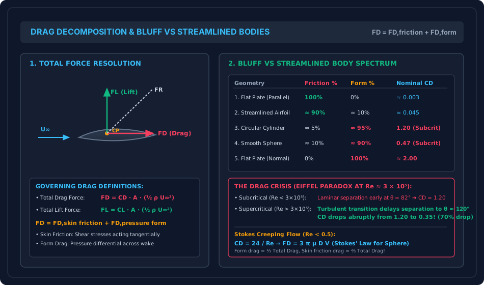
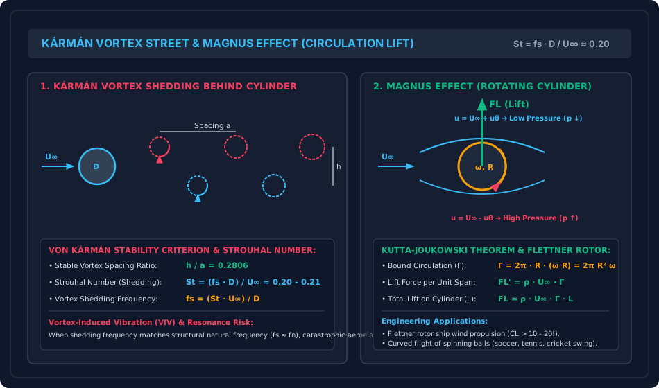
Figure 2: Von Kármán Vortex Street Dynamics & Magnus Rotor Propulsion
This schematic details the staggered vortex street topology behind a circular cylinder, the Strouhal shedding frequency relationships, structural lock-in phenomena, and the asymmetric streamline deflection causing Magnus lift on a Flettner rotor.
6. Comparative Engineering Analysis & Parameter Regimes
| Geometry / Flow Configuration | Flow Regime | Friction Drag () % | Form / Pressure Drag () % | Nominal Drag Coeff. | Separation Location | Primary Determinant of Total Drag |
|---|---|---|---|---|---|---|
| Flat Plate Parallel to Stream | Laminar () | No separation | Viscous shear stresses along wetted area | |||
| Flat Plate Parallel to Stream | Turbulent () | No separation | Turbulent wall shear stress | |||
| Streamlined Airfoil / Strut | Design Angle of Attack () | Trailing edge only | Wetted surface skin friction | |||
| Sphere in Creeping Flow | Stokes () | () | () | No wake separation | Viscous diffusion throughout entire field | |
| Circular Cylinder (Subcritical) | (Forebody) | Wide wake low base pressure deficit | ||||
| Circular Cylinder (Supercritical) | (Drag Crisis) | (Aft) | Turbulent boundary layer delaying separation | |||
| Sphere (Supercritical) | (Drag Crisis) | (Aft) | Dimpled / tripped turbulent boundary layer | |||
| Flat Plate Normal to Stream | All | Sharp edges () | Fixed geometric edge separation, constant wake |
7. Worked Numerical Examples (Pre-Calculated & Verified)
Problem 1: Industrial Chimney Subjected to Hurricane Winds & Vortex Shedding
Problem Statement: A reinforced concrete industrial chimney of uniform outer diameter and total height stands in an open coastal terrain. During a cyclonic storm, the chimney is subjected to a uniform horizontal approach wind velocity of (). Ambient air properties are and kinematic viscosity .
Given that the design drag coefficient for the cylindrical surface in this flow regime is , calculate:
- The approach Reynolds number and the state of the boundary layer.
- The total horizontal wind drag force acting on the chimney.
- The overturning bending moment exerted at the foundation base.
- The dominant periodic vortex shedding frequency and period assuming .
- The critical approach wind speed that would induce aeroelastic resonance (lock-in) if the fundamental natural flexural frequency of the chimney is .
Step-by-Step Solution:
1. Reynolds Number Calculation:
Since , the flow operates squarely in the transcritical / post-critical turbulent boundary layer regime.
2. Dynamic Wind Pressure and Frontal Area:
Frontal projected area:
3. Total Wind Drag Force ():
4. Overturning Bending Moment at Base (): Assuming uniform wind pressure along the height, the resultant horizontal drag acts at mid-height:
5. Vortex Shedding Frequency () and Period (): Using the Strouhal number relation:
The period of alternating transverse lift cycles is:
6. Critical Resonance Wind Speed (): Resonance occurs when the shedding frequency matches the structure's natural frequency ():
Engineering Note: Because is a very common gentle wind speed, the chimney will encounter frequent resonance during normal service unless fitted with helical aerodynamic strakes or tuned mass dampers.
Problem 2: Silt Settling in Water vs Parachute Descent Terminal Velocity
Problem Statement:
- Part A (Stokes Settling): A spherical fine silt particle of diameter () and specific gravity settles in still water (). Determine the terminal settling velocity , the particle Reynolds number , the Stokes drag coefficient , and verify that Stokes' law is strictly valid.
- Part B (Parachute Terminal Velocity): A parachutist with gear has a combined mass of . The hemispherical canopy has an inflated diameter of and a drag coefficient . Taking ambient air density as , compute the terminal landing descent velocity in and .
Step-by-Step Solution:
Part A: Stokes Settling of Silt Particle:
-
Diameter: .
-
Submerged buoyant weight of the spherical particle:
-
Terminal velocity from Stokes' Law:
-
Verification of Particle Reynolds Number:
Since , the flow is strictly within the creeping Stokesian regime. Stokes' law is valid.
-
Stokes Drag Coefficient:
Part B: Parachute Terminal Descent Velocity:
- Total weight: .
- Planform projected area of the circular canopy:
- Dynamic equilibrium at terminal velocity ():
- Velocity in :
Problem 3: Flettner Rotor Cargo Ship & The Magnus Effect
Problem Statement: An energy-efficient modern cargo vessel is equipped with a cylindrical Flettner rotor installed on its upper deck to provide supplementary wind propulsion. The rotor has an outer diameter (radius ) and a vertical height .
The ship encounters a crosswind relative approach velocity of in ambient air of density . The cylinder is mechanically driven to rotate at .
Calculate:
- The cylinder angular velocity , surface tangential peripheral speed , and the non-dimensional spin ratio .
- The theoretical ideal circulation generated by the rotating surface.
- The theoretical maximum Kutta-Joukowski transverse lift force .
- Given that in real viscous separated flow at this spin ratio (), experimental measurements with top disk endplates yield actual coefficients and , determine the actual Lift force , Drag force , resultant hydrodynamic force , and the angle of action relative to the wind stream.
Step-by-Step Solution:
1. Rotational Kinematics:
Peripheral surface velocity:
Spin velocity ratio:
2. Theoretical Circulation ():
3. Theoretical Kutta-Joukowski Lift Force (): Lift force per unit length:
Total theoretical lift over height :
4. Actual Hydrodynamic Forces in Real Viscous Flow: Frontal projected area:
Dynamic wind pressure:
Actual Lift Force ():
Actual Drag Force ():
Resultant Aerodynamic Force ():
Resultant Force Vector Angle ():
8. High-Yield Examination Traps & Ambiguities
- Stokes Drag Decomposition ( vs Trap):
- Trap: Confusing form drag and friction drag fractions for a sphere in creeping flow.
- Anchor: Form (pressure) drag is (), while skin friction drag is (). Many students incorrectly assume friction is and form is .
- Projected Area vs Planform Area Reference:
- Trap: Using planform area for cylinders/spheres or projected area for flat plates.
- Rule: For cylinders and spheres, always use the frontal projected area ( for cylinder, for sphere). For thin flat plates, use wetted surface area () or total surface area () depending on whether one side or both sides are exposed.
- The Drag Crisis Sign Ambiguity:
- Trap: Thinking that turbulent boundary layers always increase drag.
- Clarification: For a streamlined body (flat plate or slender airfoil), transitioning from laminar to turbulent boundary layer increases drag by because skin friction dominates. For a bluff body (cylinder or sphere), transitioning to turbulence decreases total drag by over (the Drag Crisis) because form drag dominates and turbulence delays separation.
- Vortex Shedding Frequency: Lift vs Drag Pulsation:
- Trap: Stating that drag oscillates at the vortex shedding frequency .
- Clarification: Alternating transverse Lift force oscillates at , but in-line Drag force pulsates at twice the frequency () because one vortex sheds from either the top or bottom every half cycle.
- Kármán Vortex Street Stability Ratio ():
- Trap: Inverting the ratio or using incorrect decimal approximations.
- Exact: .
9. Real-World Engineering Applications & Case Studies
- Tacoma Narrows Bridge Disaster (1940): While traditionally cited as simple vortex resonance, the catastrophic collapse of the Tacoma Narrows Bridge involved coupled aerodynamic aeroelastic flutter. Periodic vortex shedding from the bluff H-beam deck initialized vertical oscillations that locked into the torsional natural frequency of the suspension span. Modern suspension bridges utilize streamlined aerofoil-shaped hollow box girders to minimize wake separation.
- Ferrybridge Cooling Towers Collapse (UK, 1965): Three tall hyperbolic cooling towers collapsed during high winds due to group aerodynamic interference. The wakes and vortex streets shed from the windward towers increased turbulence and dynamic gust loads on the leeward towers, causing structural fatigue buckling.
- Chimney Helical Strakes (Scruton Strakes): Tall industrial chimneys, flare stacks, and rocket launch gantries are equipped with sharp-edged helical strakes. These strakes break the spanwise coherence of the boundary layer, preventing uniform simultaneous vortex shedding and suppressing cross-wind lock-in vibrations.
- Modern Flettner Rotor Ships (Norsepower Rotors): Large ocean cargo vessels are retrofitted with automated Flettner rotors. By rotating in prevailing ocean crosswinds, the rotors generate auxiliary forward propulsion thrust via the Magnus effect, reducing fuel consumption and greenhouse gas emissions by .
10. Cross-Disciplinary & Downstream Dependencies
                     ┌──────────────────────────────────────────┐
                     │ FM-07-01: Boundary Layer Development &  │
                     │ Blasius Flat Plate Solution             │
                     └────────────────────┬─────────────────────┘
                                          │
                                          ▼
                     ┌──────────────────────────────────────────┐
                     │ FM-07-02: Momentum Integral Equation &  │
                     │ Separation Hydrodynamics                 │
                     └────────────────────┬─────────────────────┘
                                          │
                                          ▼
┌────────────────────────────────────────────────────────────────────────────────────────┐
│ FM-07-03: DRAG & LIFT ON SUBMERGED BODIES, BLUFF VS STREAMLINED, VORTEX STREET, MAGNUS │
└───────────┬─────────────────────────────┬───────────────────────────────┬──────────────┘
            │                             │                               │
            ▼                             ▼                               ▼
┌───────────────────────┐   ┌───────────────────────────┐   ┌────────────────────────────┐
│ Structural Wind Load  │   │ Sediment Transport &      │   │ FM-08-01: Hydraulic Jets,  │
│ Analysis (IS 875 Pt 3)│   │ Environmental Engineering │   │ Turbines & Pumps Machinery │
│ Tall Chimneys & Masts │   │ Settling Basins (Stokes)  │   │ Blade Lift & Drag Profiles │
└───────────────────────┘   └───────────────────────────┘   └────────────────────────────┘
- Upstream: Builds directly on Blasius boundary layer scaling (
FM-07-01) and Von Kármán momentum integral separation mechanics (FM-07-02). - Downstream Structural: Crucial prerequisite for wind load design on civil infrastructure (IS 875 Part 3), bridge aerodynamics, and chimney base foundations.
- Downstream Hydraulic Machinery: Provides the aerodynamic and hydrodynamic blade foil lift/drag theory governing Pelton, Francis, and Kaplan turbine runners (
FM-08-01toFM-08-03).
11. Summary Formula Cheat Sheet & Memory Anchors
- Total Drag:
- Total Lift:
- Stokes Law (): ( pressure form, skin friction)
- Stokes Drag Coefficient:
- Stokes Particle Settling Velocity:
- Strouhal Number: (for cylinder in subcritical regime)
- Vortex Street Stability Ratio:
- Critical Wind Speed for Lock-in:
- Kutta-Joukowski Lift Theorem:
- Magnus Peripheral Speed Ratio:
12. Comprehensive References & Standard Codes
- Schlichting, H., & Gersten, K. (2017). Boundary-Layer Theory (9th ed.). Springer-Verlag, Berlin.
- White, F. M. (2016). Fluid Mechanics (8th ed.). McGraw-Hill Education, New York.
- Fox, R. W., McDonald, A. T., & Pritchard, P. J. (2015). Introduction to Fluid Mechanics (9th ed.). John Wiley & Sons.
- Modi, P. N., & Seth, S. M. (2020). Hydraulics and Fluid Mechanics Including Hydraulics Machines (22nd ed.). Standard Book House, New Delhi.
- IS 875 (Part 3): 2015 — Design Loads (Other Than Earthquake) For Buildings and Structures — Code of Practice: Part 3 Wind Loads. Bureau of Indian Standards, New Delhi.
- Blevins, R. D. (1990). Flow-Induced Vibration (2nd ed.). Van Nostrand Reinhold, New York.