Particle Acceleration — Substantial Derivative, Local vs Convective Acceleration & Natural Coordinates
In this chapter (5 topics)
On this page
- 1. Topic Metadata Table
- 2. Executive Summary
- 3. Substantial / Material Derivative Operator
- 3.1 Lagrangian Tracking in an Eulerian Field
- 3.2 Operator Definition
- 4. Decomposition of Fluid Particle Acceleration in Cartesian Coordinates
- 4.1 Component-Wise Expressions
- 4.2 Resultant Total Acceleration Magnitude & Direction
- 5. 4-Quadrant Acceleration Classification Matrix
- Detailed Flow Regime Characteristics
- 6. Particle Acceleration in Natural / Streamline Coordinates (s, n)
- 6.1 Coordinate Definitions
- 6.2 Acceleration Derivation
- 6.3 Physical Roles of at and an
- 7. Civil Engineering Applications
- 7.1 Transverse Water Surface Super-Elevation in Canal Bends
- 7.2 Dynamic Reaction & Thrust Blocks in Pipe Bends
- 8. Visual Diagrams & Architectural Schematics
- 8.1 Substantial Derivative & Local vs Convective Acceleration
- 8.2 Natural Coordinates Geometry & Canal Bend Super-Elevation
- 9. Step-by-Step Numerical Problems with Complete Calculations
- Problem 1: Complete 3D Unsteady Acceleration Decomposition
- Problem 2: Linearly Converging Circular Nozzle with Unsteady Discharge
- Problem 3: Acceleration in a Curved Canal Bend in Natural Coordinates
- 10. High-Yield Exam Pitfalls, Traps & Shortcuts
- 11. Multi-Exam Question Bank (GATE, ESE, SSC JE, State AE, RRB JE)
- Question 1 (GATE CE — Analytical)
- Question 2 (UPSC ESE Paper-II — Descriptive / Analytical)
- Question 3 (SSC JE — Conceptual)
- Question 4 (State PSC AE — Numerical)
- Question 5 (RRB JE — Direct Knowledge)
- 12. Comprehensive Summary, Formula Cheatsheet & Academic References
- 12.1 Formula Cheatsheet
- 12.2 Academic & Standard References
1. Topic Metadata Table
| Field | Detail |
|---|---|
| Subject | Fluid Mechanics & Hydraulic Machinery (Subject 07) |
| Chapter | Chapter 03: Fluid Kinematics |
| Topic Code | FM-03-03 |
| Topic Title | Particle Acceleration: Substantial Derivative, Local (Temporal) vs Convective Acceleration, Acceleration in Natural Coordinates () |
| Prerequisites | FM-03-01 (Flow Classification, Streamlines & Pathlines), FM-03-02 (Continuity Equation), Vector Calculus (Directional Derivative, Gradient Operator) |
| Target Examinations | GATE CE, UPSC ESE (Paper-II), SSC JE, State PSC AE/JE, RRB JE |
| Knowledge Level | Fundamental Kinematic Derivation to Advanced Field Analysis |
| IS / IRC / Standard Codes | IS 4880 (Code of practice for design of tunnels, hydraulic aspects), IS 7784 (Design of canal transitions) |
| Key Formulae | , , , |
2. Executive Summary
In solid mechanics, tracking the acceleration of a rigid body or mass point is straightforward because the coordinate system is naturally attached to the particle (Lagrangian approach: ). In continuum fluid mechanics, however, velocities are mapped as continuous vector fields at fixed spatial stations (Eulerian approach: ). Consequently, to determine the true Newton's second law acceleration experienced by a moving fluid parcel, one must calculate the Total (Substantial or Material) Derivative of the velocity vector:
This fundamental decomposition divides fluid acceleration into two distinct physical mechanisms:
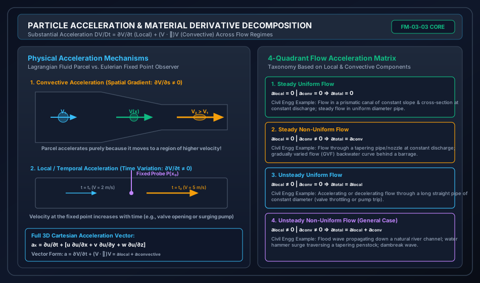
- Local (Temporal) Acceleration (): The time rate of change of fluid velocity at a fixed spatial coordinate. This component is non-zero exclusively in unsteady flow (e.g., during valve throttling, pump tripping, or flood wave propagation) and vanishes identically in all steady flows.
- Convective Acceleration (): The rate of change of velocity resulting from the spatial displacement of a fluid parcel through a non-uniform velocity field. This component is non-zero exclusively in non-uniform flow (e.g., fluid traversing converging nozzles, diffusers, bends, or gradually varied open channels) and vanishes in uniform flow.
When fluid parcels travel along curved trajectories, Cartesian coordinates obscure the physical nature of motion. We project acceleration onto Natural (Streamline) Coordinates , where is the arc-length along the streamline and is the normal directed toward the center of curvature. The acceleration splits into:
- Tangential Acceleration (): Governs changes in the magnitude of speed along the streamline:
- Normal (Centripetal) Acceleration (): Governs changes in the direction of the velocity vector toward the local center of curvature of radius :
A crucial civil engineering consequence of normal acceleration is the lateral pressure gradient that induces super-elevation of the water surface in canal bends (), creates dynamic thrust on pipe bends requiring anchor blocks, and drives helical secondary currents responsible for outer bank scour and inner bank point-bar deposition in alluvial rivers.
3. Substantial / Material Derivative Operator
To track how any fluid property (scalar like pressure , temperature , or density ; or vector like velocity ) changes for a specific fluid particle as it migrates through space, we use the chain rule of multivariable calculus.
3.1 Lagrangian Tracking in an Eulerian Field
Let the spatial position of a fluid parcel at time be given by . By definition of particle velocity:
Now let be any continuous differentiable fluid field property. The total differential experienced by the moving particle in time is:
Dividing by the elapsed time increment :
Substituting the velocity components :
3.2 Operator Definition
The Material (Substantial, Total, or Particle) Derivative Operator is denoted by :
Here:
- is the Local / Temporal Derivative (measured by a stationary Eulerian probe).
- is the Convective Derivative Operator (induced by particle translation across spatial gradients).
4. Decomposition of Fluid Particle Acceleration in Cartesian Coordinates
Applying the substantial derivative operator directly to the velocity vector :
In 3D Cartesian coordinates, the particle acceleration vector is resolved into three scalar components:
4.1 Component-Wise Expressions
1. -Component of Acceleration ():
2. -Component of Acceleration ():
3. -Component of Acceleration ():
4.2 Resultant Total Acceleration Magnitude & Direction
The resultant particle acceleration magnitude is:
The direction cosines with respect to the axes are:
5. 4-Quadrant Acceleration Classification Matrix
The existence of local versus convective acceleration creates four distinct flow regimes that form the cornerstone of hydraulic classification:
                              FLOW REGIME CLASSIFICATION
                                          │
                  ┌───────────────────────┴───────────────────────┐
                  ▼                                               ▼
             STEADY FLOW                                    UNSTEADY FLOW
         (∂V/∂t = 0 => a_local = 0)                   (∂V/∂t ≠ 0 => a_local ≠ 0)
                  │                                               │
        ┌─────────┴─────────┐                           ┌─────────┴─────────┐
        ▼                   ▼                           ▼                   ▼
     UNIFORM           NON-UNIFORM                   UNIFORM           NON-UNIFORM
   (∂V/∂s = 0)         (∂V/∂s ≠ 0)                 (∂V/∂s = 0)         (∂V/∂s ≠ 0)
        │                   │                           │                   │
  a_conv = 0          a_conv ≠ 0                  a_conv = 0          a_conv ≠ 0
  a_total = 0        a_total = a_conv            a_total = a_local   a_total = a_loc + a_conv
Detailed Flow Regime Characteristics
| Regime | Local Accel () | Convective Accel () | Total Accel () | Typical Civil Engineering Hydraulics Example |
|---|---|---|---|---|
| 1. Steady Uniform Flow | Constant discharge in a straight, prismatic canal of uniform cross-section and slope; laminar or turbulent flow through a uniform diameter pipe at constant pump head. | |||
| 2. Steady Non-Uniform Flow | Constant discharge through a tapering pipe, nozzle, or venturimeter; gradually varied flow (GVF) backwater curve created upstream of a barrage or dam; flow over a broad-crested weir. | |||
| 3. Unsteady Uniform Flow | Accelerating or decelerating flow in a long straight pipeline of constant diameter during valve opening/closing; surging flow in a uniform canal where discharge varies with time. | |||
| 4. Unsteady Non-Uniform Flow | Propagation of a flood wave or dambreak bore in a natural meandering river channel; water hammer pressure transients traveling along a tapering penstock. |
6. Particle Acceleration in Natural / Streamline Coordinates ()
In many curved hydraulic structures—such as canal bends, spillway ski-jump buckets, radial gates, and river meanders—Cartesian coordinates obscure the direct relationship between speed changes and directional turning. We establish an intrinsic orthogonal coordinate system tied to the streamline.
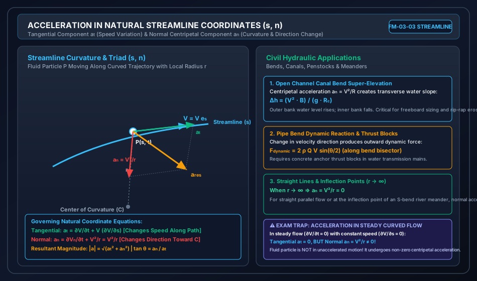
                            ^ e_s (Unit Tangent)
                           /
                          /  V = V e_s
                         /
             ───────────●────────────────> Streamline s
                       /│ P(s,t)
                      / │
                     /  │
                    /   │ e_n (Unit Normal pointing to C)
                   /    ▼
                  /
                 /  Radius of Curvature r
                /
               ● Center of Curvature C
6.1 Coordinate Definitions
- : Arc length measured along the streamline in the direction of flow.
- : Normal distance measured perpendicular to the streamline, directed inward toward the local center of curvature .
- : Unit tangent vector along the streamline ().
- : Unit normal vector pointing toward the center of curvature.
- : Local radius of curvature of the streamline ().
By definition, the velocity vector is strictly tangent to the streamline at all times:
Notice that there is no normal component of velocity across a streamline ().
6.2 Acceleration Derivation
Differentiating the velocity vector with respect to time for a moving parcel:
-
Substantial Derivative of Speed ():
This is the Tangential Acceleration Component ():
-
Rate of Change of Unit Tangent Vector (): As the fluid parcel traverses an arc length , the direction of the unit tangent vector rotates by an angle :
The change vector points perpendicular to , directly toward the center of curvature, along :
Applying the chain rule:
Substituting back into the acceleration equation:
This is the Normal / Centripetal Acceleration Component ():
6.3 Physical Roles of and
- changes the magnitude of velocity (speed): If , the fluid parcel speeds up; if , it slows down.
- changes the direction of velocity: Even if the flow is steady () and has constant speed along the streamline (), as long as the path is curved ().
- Resultant Acceleration: Angle of resultant acceleration vector relative to streamline tangent:
7. Civil Engineering Applications
7.1 Transverse Water Surface Super-Elevation in Canal Bends
When water at mean velocity negotiates a canal bend of width and centerline radius , every fluid parcel undergoes inward normal acceleration . By Newton's second law, this centripetal acceleration requires an inward radial pressure gradient:
For hydrostatic pressure distribution :
Integrating across the canal width from the inner bank to the outer bank ():
Practical Significance:
- The water surface tilts upward at the outer bank and downward at the inner bank.
- The outer bank requires increased freeboard and stone pitching (rip-rap) to prevent overtopping and erosion.
- Near the canal bed, boundary layer friction reduces the longitudinal velocity (), while the lateral pressure gradient remains nearly uniform. This imbalance drives a secondary transverse helical circulation that carries bed sediment toward the inner bank (forming point bars) and erodes the outer bank toe.
7.2 Dynamic Reaction & Thrust Blocks in Pipe Bends
When water flows through a pipe bend of angle , the normal acceleration redirects the fluid momentum vector, exerting a dynamic outward thrust on the pipe wall:
Together with the hydrostatic pressure thrust , this combined force requires a cast-in-place concrete thrust block anchored into solid ground to prevent joint pullout.
8. Visual Diagrams & Architectural Schematics
8.1 Substantial Derivative & Local vs Convective Acceleration
The diagram below illustrates the physical decomposition between an Eulerian fixed-point velocity sensor (local acceleration ) and a moving Lagrangian parcel navigating a spatial gradient (convective acceleration ), accompanied by the 4-quadrant flow classification matrix.
8.2 Natural Coordinates Geometry & Canal Bend Super-Elevation
The schematic below presents the natural coordinate triad on an intrinsic curved streamline, delineating tangential acceleration and normal centripetal acceleration , alongside civil hydraulic engineering applications in canal bends and thrust blocks.
9. Step-by-Step Numerical Problems with Complete Calculations
Problem 1: Complete 3D Unsteady Acceleration Decomposition
Problem Statement: The velocity field of an unsteady 3D fluid flow is defined by:
where coordinates are in meters, time in seconds, and velocity components in . At the point and time :
- Compute the local acceleration vector and its magnitude.
- Compute the convective acceleration vector and its magnitude.
- Compute the total acceleration vector and its magnitude.
Step 1: Evaluate Velocity Components at at
Step 2: Compute Local (Temporal) Acceleration Vector
The local acceleration components are :
Therefore:
Step 3: Compute Convective Acceleration Vector
First, evaluate the spatial derivatives at :
Now evaluate the convective acceleration components:
Therefore:
Step 4: Compute Total Acceleration Vector
Problem 2: Linearly Converging Circular Nozzle with Unsteady Discharge
Problem Statement: Water flows through a horizontally mounted converging circular pipe of axial length . The inlet diameter is at , and the outlet diameter is at . The diameter tapers linearly:
Due to opening of an upstream regulating valve, the volumetric discharge increases linearly with time according to:
where and . At time , evaluate at the midpoint of the nozzle ():
- The local acceleration .
- The convective acceleration .
- The total acceleration .
Step 1: Geometric & Discharge Values at and
Diameter at midpoint :
Cross-sectional area at midpoint:
Discharge at :
Mean flow velocity at midpoint:
Step 2: Compute Local Acceleration
Local acceleration is the partial time derivative of velocity at fixed :
Given , .
Step 3: Compute Convective Acceleration
Convective acceleration along the -axis is:
Since :
Here, . Substituting values:
Now compute :
Step 4: Compute Total Acceleration
Key Insight: Convective acceleration accounts for of the total acceleration, illustrating that geometric constriction dominates over temporal surging in this transition.
Problem 3: Acceleration in a Curved Canal Bend in Natural Coordinates
Problem Statement: A trapezoidal open irrigation canal incorporates a horizontal curve with centerline radius of curvature . Water flows through the bend such that its speed increases linearly along the streamline:
where is the arc length from the start of the curve (), , and . Due to upstream sluice adjustments, water speed is also accelerating with time at a uniform rate:
At a station along the curve:
- Determine the tangential acceleration component .
- Determine the normal centripetal acceleration component .
- Determine the resultant total acceleration magnitude and its angle with respect to the streamline tangent.
Step 1: Compute Speed at
The spatial gradient along the streamline is:
Step 2: Compute Tangential Acceleration
Step 3: Compute Normal Acceleration
The normal acceleration is centripetal toward the center of curvature:
Step 4: Compute Resultant Acceleration & Direction
Angle relative to the forward streamline tangent:
The resultant acceleration vector acts at an angle of inward from the forward tangent toward the center of curvature.
10. High-Yield Exam Pitfalls, Traps & Shortcuts
- The Classic Steady Flow Trap:
- False belief: "If the flow is steady, acceleration is always zero."
- Reality: In steady flow, only local acceleration is zero (). If the flow is non-uniform (e.g., flow through a nozzle, bend, or over a weir), convective acceleration is non-zero (). The total acceleration is therefore non-zero!
- The Steady Curved Flow Trap:
- False belief: A fluid particle moving at constant speed along a curved path of constant radius has zero acceleration.
- Reality: Tangential acceleration is zero (), but normal acceleration is non-zero (). The particle is continually accelerated inward.
- Difference Between 1D Cartesian and Natural Coordinates:
- In 1D Cartesian flow (), convective acceleration is .
- In natural coordinates along a streamline, convective tangential acceleration is , while normal acceleration is .
- Inflection Points in Meanders:
- At the inflection point of an S-shaped meandering river channel, the radius of curvature approaches infinity (). Consequently, the normal acceleration vanishes identically (). The flow at the inflection point experiences only tangential acceleration.
- Quick Shortcut for Uniform Flow:
- Whenever a question specifies "uniform pipe of constant cross-section", all convective spatial derivatives vanish: . The total acceleration is simply the local time derivative .
11. Multi-Exam Question Bank (GATE, ESE, SSC JE, State AE, RRB JE)
Question 1 (GATE CE — Analytical)
For a two-dimensional flow field given by , the convective acceleration vector at the point is:
(A)
(B)
(C)
(D)
Solution: Here, and . At :
Evaluate spatial derivatives at :
Convective acceleration components:
Correct Option: (B)
Question 2 (UPSC ESE Paper-II — Descriptive / Analytical)
Water flows through a duct such that the velocity is given by . The convective acceleration at and is:
(A)
(B)
(C)
(D)
Solution: Here, . At and :
Spatial derivative:
At :
Convective acceleration:
(Note: If asked for local acceleration: ). Correct Option: (B)
Question 3 (SSC JE — Conceptual)
Convective acceleration is defined as the rate of change of velocity due to the change of:
(A) Position of fluid particles in a fluid flow
(B) Properties of fluid with time
(C) Temperature of the fluid
(D) Pressure head with time
Solution:
Convective acceleration is the component of total acceleration caused by the spatial displacement of a fluid parcel as it travels between points of different velocity in a non-uniform flow field. Local acceleration is due to the change with time at a fixed location.
Correct Option: (A)
Question 4 (State PSC AE — Numerical)
In a steady flow through a nozzle, the velocity varies along the axis as , where is the distance from the inlet in meters. The acceleration of a fluid particle at is:
(A)
(B)
(C)
(D)
Solution: Flow is steady . The flow is 1D . Given :
At :
Correct Option: (B)
Question 5 (RRB JE — Direct Knowledge)
When a fluid particle moves along a curved path with a constant speed, its:
(A) Both tangential and normal accelerations are zero
(B) Tangential acceleration is zero, but normal acceleration is non-zero
(C) Tangential acceleration is non-zero, but normal acceleration is zero
(D) Resultant acceleration is zero
Solution:
Constant speed and .
Curved path .
Thus, tangential acceleration is zero, but normal (centripetal) acceleration is non-zero.
Correct Option: (B)
12. Comprehensive Summary, Formula Cheatsheet & Academic References
12.1 Formula Cheatsheet
┌────────────────────────────────────────────────────────────────────────────────────────┐
│                        PARTICLE ACCELERATION CHEATSHEET                                │
├────────────────────────────────────────────────────────────────────────────────────────┤
│ 1. Substantial Derivative Operator:                                                    │
│    D/Dt = ∂/∂t + u ∂/∂x + v ∂/∂y + w ∂/∂z = ∂/∂t + (V·∇)                               │
│                                                                                        │
│ 2. Total Acceleration Vector:                                                          │
│    a = DV/Dt = a_local + a_convective = ∂V/∂t + (V·∇)V                                 │
│                                                                                        │
│ 3. Cartesian Scalar Components:                                                        │
│    ax = ∂u/∂t + [u ∂u/∂x + v ∂u/∂y + w ∂u/∂z]                                          │
│    ay = ∂v/∂t + [u ∂v/∂x + v ∂v/∂y + w ∂v/∂z]                                          │
│    az = ∂w/∂t + [u ∂w/∂x + v ∂w/∂y + w ∂w/∂z]                                          │
│    |a| = √(ax² + ay² + az²)                                                            │
│                                                                                        │
│ 4. Natural (Streamline) Coordinates (s, n):                                            │
│    Tangential: at = ∂V/∂t + V (∂V/∂s)   [Governs rate of change of speed]              │
│    Normal:     an = ∂Vn/∂t + V²/r = V²/r [Centripetal; inward toward C]                │
│    Resultant:  |a| = √(at² + an²),   tan θ = an / at                                   │
│                                                                                        │
│ 5. Curvature Special Conditions:                                                       │
│    Straight Streamline: r -> ∞ => an = 0                                               │
│    Inflection Point:    r -> ∞ => an = 0                                               │
│    Canal Bend Super-Elevation: Δh = (V² · B) / (g · R_c)                               │
└────────────────────────────────────────────────────────────────────────────────────────┘
12.2 Academic & Standard References
- White, F. M. (2016). Fluid Mechanics (8th ed.). McGraw-Hill Education, New York. (Chapter 4: Differential Relations for Fluid Flow — Substantial Derivative and Acceleration Field).
- Fox, R. W., McDonald, A. T., & Pritchard, P. J. (2015). Introduction to Fluid Mechanics (9th ed.). John Wiley & Sons. (Kinematics of Fluid Motion).
- Modi, P. N., & Seth, S. M. (2018). Hydraulics and Fluid Mechanics Including Hydraulics Machines (22nd ed.). Standard Book House, New Delhi. (Chapter 5: Fluid Kinematics & Particle Acceleration).
- Subramanya, K. (2018). Theory and Applications of Fluid Mechanics. Tata McGraw-Hill, New Delhi.
- Bureau of Indian Standards. IS 7784: Code of Practice for Design of Canal Transitions. New Delhi, India.