Fluid Properties, Continuum Hypothesis & Newton's Law of Viscosity
In this chapter (4 topics)
On this page
- 1. Topic Metadata & Syllabus Mapping
- 2. Executive Summary & Core Engineering Concepts
- 2.1 The Continuum Hypothesis
- 3. Comprehensive Technical Principles & Mechanics
- 3.1 Primary Fluid Properties
- 3.2 Dynamic (Absolute) Viscosity (μ)
- 3.3 Kinematic Viscosity (ν)
- 3.4 Physical Mechanisms of Temperature Dependence
- 4. Detailed Technical Diagrams & Visual Models
- 4.1 Shear Strain Kinematics & Couette Flow
- 4.2 Temperature Dependence & Viscosity Conversion Matrix
- 5. Comprehensive Step-by-Step Mathematical Derivations
- 5.1 Derivation of Newton's Law of Viscosity (dθ/dt = du/dy)
- 5.2 Torque and Power Dissipation in a Concentric Cylinder Viscometer
- 5.3 Viscous Torque on a Rotating Circular Collar / Pivot Bearing
- 6. Three Fully Worked Unit-Checked Numerical Examples
- Example 1: Sliding Plate on an Inclined Lubricated Plane
- Example 2: Rotating Shaft in Sleeve Bearing (Journal Bearing Viscometer)
- Example 3: Rotating Flat Collar Bearing with Radial Viscous Dissipation
- 7. Common Engineering Pitfalls & Examination Traps
- 8. Real-World Case Studies & Industrial Applications
- Hydrodynamic Lubrication & the 1905 Kingsbury Thrust Bearing Revolution
- 9. Competitive Examination Practice Problems
- Problem 1 (GATE CE - 1 Mark)
- Problem 2 (UPSC ESE Paper-II - 2 Marks)
- Problem 3 (SSC JE - 1 Mark)
- Problem 4 (State PSC AE - 2 Marks)
- Problem 5 (RRB JE - 1 Mark)
- 10. Cross-Subject Synthesis & Advanced Fluid Couplings
- 11. Standard Reference Textbooks & Official Code Specifications
- 12. Comprehensive Summary, Formula Cheatsheet & Key Takeaways
1. Topic Metadata & Syllabus Mapping
| Attribute | Specification |
|---|---|
| Module / Topic ID | FM-01-01 |
| Subject | Fluid Mechanics & Hydraulic Machinery |
| Chapter | 01: Fluid Properties & Rheology |
| Topic Title | Fluid Properties, Continuum Hypothesis & Newton's Law of Viscosity |
| Primary Reference Standards | IS 4987, ISO 3104 (Petroleum products - Kinematic viscosity), Frank M. White (Fluid Mechanics), Fox & McDonald (Introduction to Fluid Mechanics), Modi & Seth (Hydraulics and Fluid Mechanics) |
| Target Competitive Examinations | GATE CE, UPSC ESE (Paper-II), SSC JE, State PSC AE/JE, RRB JE |
| Examination Weightage | GATE (1 to 2 Marks), UPSC ESE (4 to 8 Marks prelims/mains), SSC JE (2 to 4 Marks), State AE/JE (2 to 4 Marks) |
| Prerequisites | Engineering Mechanics (Equilibrium of Forces), Calculus (Differential Equations) |
2. Executive Summary & Core Engineering Concepts
In civil and mechanical engineering, a fluid is defined as a substance that deforms continuously and permanently under the application of any shear stress, however small. Unlike a solid, which resists an applied shear stress by undergoing a finite elastic deformation proportional to the shear stress (), a fluid continuously deforms at a strain rate proportional to the applied shear stress (). A fluid at rest cannot sustain any shear stress; all internal stresses are purely normal compressive pressures.
+-----------------------------------------------------------------------------------+
| DISTINCTION BETWEEN SOLID AND FLUID:                                              |
| Solid: Resists shear by static deformation -> tau = G * gamma                     |
| Fluid: Deforms continuously under shear   -> tau = mu * (d_theta / dt) = mu * du/dy|
+-----------------------------------------------------------------------------------+
2.1 The Continuum Hypothesis
At a microscopic level, fluids consist of discrete molecules moving in random thermal motion separated by empty space. For engineering analyses, the fluid is treated as a continuous macroscopic distribution of matter—a continuum—where properties such as density, velocity, pressure, and viscosity are smooth, continuously differentiable point functions.
- The validity of the continuum model is governed by the Knudsen Number (): where is the molecular mean free path (average distance travelled by a molecule between successive collisions, for air at NTP) and is the characteristic physical dimension of the flow domain.
- Continuum Regime: When , molecular fluctuations average out, and the continuum equations (Navier-Stokes) are valid.
- Slip / Free Molecular Regime: When (e.g., highly rarefied gas dynamics, re-entry vehicles in outer space, or ultra-fine MEMS micro-channels), the continuum assumption fails, and molecular kinetics must be applied.
3. Comprehensive Technical Principles & Mechanics
3.1 Primary Fluid Properties
-
Mass Density (): Mass per unit volume of fluid:
- SI Unit: . Dimensions: .
- For pure water at standard temperature () and atmospheric pressure: .
- For standard air at and : .
-
Specific Weight / Unit Weight ( or ): Gravitational force exerted per unit volume:
- SI Unit: . Dimensions: .
- For water at : .
-
Specific Volume (): Volume occupied per unit mass:
- SI Unit: . Dimensions: .
-
Specific Gravity ( or ): Dimensionless ratio of the mass density (or specific weight) of the given fluid to that of a standard reference fluid at standard temperature:
- For liquids: Standard reference fluid is pure water at ():
- For gases: Standard reference fluid is dry air at and ():
- Benchmarks: Mercury (), Standard lubricating oil (), Gasoline ().
3.2 Dynamic (Absolute) Viscosity ()
Viscosity is the internal property of a fluid that offers resistance to relative deformation, shear strain, and sliding between adjacent fluid layers.
Newton's Law of Viscosity:
In a laminar parallel shear flow, the shear stress () acting on a fluid plane is directly proportional to the rate of angular deformation (shear strain rate ), which equals the transverse velocity gradient ():
Where:
- = Shear stress parallel to the direction of flow ( or ).
- = Velocity gradient perpendicular to the direction of motion ().
- = Coefficient of dynamic viscosity (or absolute viscosity).
Units and Dimensions of Dynamic Viscosity:
- Dimensions: or .
- SI Unit: ().
- CGS Unit: Poise (P), named after Jean Léonard Marie Poiseuille:
- Conversion Factor: Key Exam Fact: Water at has .
3.3 Kinematic Viscosity ()
Kinematic viscosity represents the momentum diffusivity of a fluid—the ratio of the internal resistance force to the inertial force of the fluid:
Units and Dimensions of Kinematic Viscosity:
- Note that kinematic viscosity contains no mass or force dimension; it is purely geometric and temporal!
- SI Unit: .
- CGS Unit: Stoke (St), named after Sir George Gabriel Stokes: Key Exam Fact: Water at has .
3.4 Physical Mechanisms of Temperature Dependence
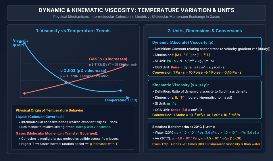
The response of viscosity to temperature variation differs fundamentally between liquids and gases due to their contrasting microscopic states of matter:
+-----------------------------------------------------------------------------------+
| PHYSICAL ORIGIN OF VISCOSITY:                                                     |
|                                                                                   |
| 1. LIQUIDS: Dominated by Intermolecular Cohesion.                                 |
|    - Molecules are tightly packed with strong cohesive intermolecular forces.    |
|    - As Temperature increases: Molecules gain kinetic energy and move apart;     |
|      intermolecular cohesion drops drastically.                                   |
|    - RESULT: Dynamic viscosity mu DECREASES exponentially: mu = D * e^(B/T).      |
|      Since liquid density rho changes very little, kinematic viscosity nu         |
|      ALSO DECREASES.                                                              |
|                                                                                   |
| 2. GASES: Dominated by Molecular Momentum Exchange.                               |
|    - Molecules are widely separated; intermolecular cohesion is negligible.       |
|    - Viscous shear arises from random thermal collisions transferring momentum    |
|      across adjacent fluid layers moving at different bulk velocities.            |
|    - As Temperature increases: Molecular thermal velocity increases (v_rms ~ sqrt(T))|
|      and collision frequency rises, enhancing momentum transfer.                  |
|    - RESULT: Dynamic viscosity mu INCREASES: mu ~ T^0.5 (Sutherland's Equation).   |
|      Furthermore, because gas density rho ~ 1/T decreases, kinematic viscosity    |
|      nu = mu / rho INCREASES EVEN FASTER with temperature!                        |
+-----------------------------------------------------------------------------------+
4. Detailed Technical Diagrams & Visual Models
4.1 Shear Strain Kinematics & Couette Flow
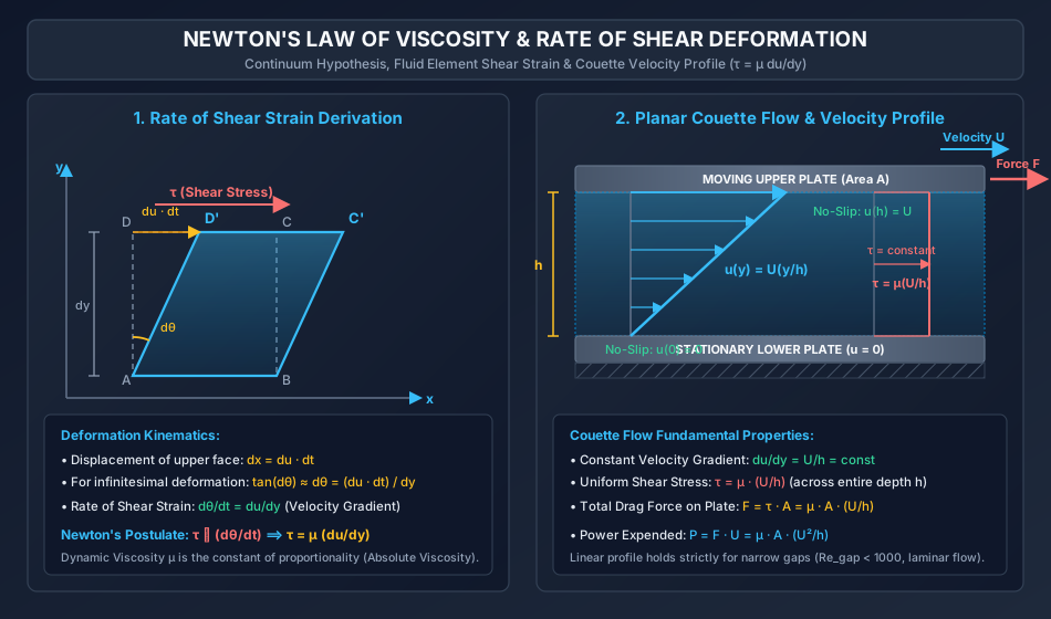
The following hand-coded engineering diagram displays the geometric derivation of the rate of shear strain () on a microscopic fluid element, and the resulting linear velocity profile and uniform shear stress distribution in laminar planar Couette flow.
4.2 Temperature Dependence & Viscosity Conversion Matrix
The following diagram illustrates the divergent trends of viscosity with temperature for liquids versus gases, highlighting the underlying molecular mechanisms (cohesion vs momentum exchange), along with the complete units conversion matrix.
5. Comprehensive Step-by-Step Mathematical Derivations
5.1 Derivation of Newton's Law of Viscosity ()
Consider a microscopic fluid element of dimensions bounded by vertices , , , and in a two-dimensional parallel shear flow .
- The lower face moves with horizontal velocity .
- The upper face , located at vertical distance above , moves with horizontal velocity , where .
- During an infinitesimal time interval :
- Point translates horizontally by distance:
- Point translates horizontally by distance:
- Relative horizontal displacement of face with respect to face :
The vertical line segment tilts through an angular displacement :
For infinitesimal angles, (in radians):
Dividing by the time interval :
Physical Conclusion: The rate of angular deformation (rate of shear strain ) of a fluid particle is mathematically identical to the transverse velocity gradient ().
Isaac Newton postulated that for simple fluids, the applied shear stress is linearly proportional to the rate of shear strain:
5.2 Torque and Power Dissipation in a Concentric Cylinder Viscometer
Consider an inner solid cylinder of radius , length , rotating at constant angular velocity () inside a stationary coaxial outer cylinder of inner radius . The radial annular gap is very small: . The clearance is filled with a Newtonian fluid of dynamic viscosity .
-
Velocity Gradient across Gap: Due to the no-slip boundary condition:
- At inner cylinder surface ():
- At outer cylinder surface (): Because the radial gap is narrow (), the velocity distribution across the gap is linear:
-
Viscous Shear Stress on Inner Cylinder Surface:
-
Viscous Tangential Drag Force: The wetted cylindrical surface area is :
-
Viscous Resisting Torque: Torque equals force multiplied by radius ():
-
Power Expended against Viscous Dissipation:
Substituting :
5.3 Viscous Torque on a Rotating Circular Collar / Pivot Bearing
Consider a flat circular disc of outer radius and inner radius (for a solid disc, ) rotating at angular speed over a stationary flat base separated by a uniform lubricant film of thickness .
- Velocity at Radius :
- Local Shear Stress:
- Shear Force on an Elemental Annular Ring of Radius and Width : Elemental area:
- Resisting Torque on Elemental Ring:
- Total Resisting Torque on Collar Bearing:
For a solid solid circular disc of radius ():
Power consumed:
6. Three Fully Worked Unit-Checked Numerical Examples
Example 1: Sliding Plate on an Inclined Lubricated Plane
Problem Statement:
A flat square steel plate of dimensions weighing slides down a plane inclined at to the horizontal. A uniform lubricating oil film of thickness separates the plate from the plane. The plate attains a uniform steady-state terminal velocity .
- Determine the dynamic viscosity of the lubricating oil in and in Poise.
- If the oil has a specific gravity , determine the kinematic viscosity in and Stokes.
Step-by-Step Solution:
Step 1: Free-Body Force Equilibrium The plate slides down the inclined plane at constant terminal velocity (). By Newton's First Law, the component of gravity down the incline is balanced by the viscous drag force acting on the bottom surface of the plate:
Step 2: Viscous Force and Dynamic Viscosity Wetted surface area of plate:
Thickness of oil film:
Assuming a linear velocity profile across the narrow oil film:
Total viscous resisting force:
Equating to the gravity driving force:
Converting to Poise ():
Step 3: Kinematic Viscosity Density of oil:
Kinematic viscosity:
Converting to Stokes ():
Example 2: Rotating Shaft in Sleeve Bearing (Journal Bearing Viscometer)
Problem Statement:
A solid steel shaft of diameter () and length () rotates inside a stationary sleeve bearing of internal diameter . The shaft rotates at a constant speed of . The uniform annular clearance between the shaft and the sleeve is filled with a lubricating oil of dynamic viscosity and specific gravity .
- Calculate the tangential shear stress developed on the surface of the shaft.
- Determine the total viscous resisting torque in .
- Determine the power lost in overcoming viscous friction in .
- Compute the kinematic viscosity in and Centistokes.
Step-by-Step Solution:
Step 1: Geometric and Kinematic Parameters
- Shaft radius:
- Radial clearance:
- Angular velocity of shaft:
- Tangential surface velocity of shaft:
Step 2: Shear Stress on Shaft Surface Assuming a linear velocity profile across the narrow radial clearance :
Step 3: Resisting Torque Wetted cylindrical surface area of the journal:
Viscous shear force:
Viscous resisting torque:
Step 4: Power Lost in Friction
Step 5: Kinematic Viscosity
In Stokes and Centistokes:
Example 3: Rotating Flat Collar Bearing with Radial Viscous Dissipation
Problem Statement:
A flat horizontal circular disc of diameter () rotates at over a stationary flat plate. The uniform clearance between the disc and the stationary plate is and is completely filled with an oil of dynamic viscosity .
- Derive the expression for the resisting torque and calculate its value.
- Calculate the power absorbed in overcoming viscous resistance.
Step-by-Step Solution:
Step 1: Kinematics and Local Shear Stress
- Angular velocity:
- At any arbitrary radius (), the local linear speed is .
- Local velocity gradient across the vertical oil film of thickness :
- Local shear stress on the underside of the rotating disc:
Step 2: Integration for Total Viscous Torque Consider an elemental annular ring of radius and radial width . Elemental area:
Viscous tangential drag on the annular ring:
Elemental resisting torque about the central axis of rotation:
Integrating from to :
Substituting the numerical parameters:
Step 3: Power Absorbed
7. Common Engineering Pitfalls & Examination Traps
| Pitfall / Exam Trap | Erroneous Concept | Correct Physical & Code Principle |
|---|---|---|
| Trap 1: Believing Water is More Kinematically Viscous than Air | Assuming that since water is denser and stickier (), its kinematic viscosity must also be higher. | While , water density () is times higher than air (). Therefore, , which is 15 times higher than that of water ()! |
| Trap 2: Confusing Temperature Effects on Gas vs Liquid Viscosity | Applying "viscosity decreases with temperature" universally to all fluids. | True for liquids (intermolecular cohesion weakens with heating). False for gases! In gases, dynamic viscosity increases with temperature because molecular momentum exchange increases (). |
| Trap 3: CGS vs SI Viscosity Unit Confusion | Forgetting the factor between Poise and . | . For kinematic viscosity, . |
| Trap 4: Neglecting the Factor of 2 in Diametral Clearance | Using directly as the gap thickness . | Clearance is radial: . Using the diametral clearance halves the calculated shear stress and torque! |
| Trap 5: Assuming Fluids at Rest Sustain Shear Stress | Believing static fluids can sustain small shear stresses like soft solids. | By definition, a fluid at rest has zero shear stress (). Any non-zero shear stress immediately induces continuous flow and deformation. |
8. Real-World Case Studies & Industrial Applications
Hydrodynamic Lubrication & the 1905 Kingsbury Thrust Bearing Revolution
- Historical Failure Context: In 19th-century steamships and hydro-turbines, propeller shafts and heavy vertical generators rode on bronze collar bearings experiencing catastrophic overheating, metal-on-metal galling, and seizure under loads exceeding .
- Fluid Mechanics Breakthrough: Albert Kingsbury and Anthony Michell demonstrated that by mounting bearing pads on pivots, the viscous dragging of oil creates a convergent wedge. Hydrodynamic pressure within the fluid film rises dynamically to several megapascals per Reynolds lubrication equation:
- Result: The shaft floats on a self-generated fluid film () with zero solid-to-solid contact. Friction coefficient dropped by (from to ), revolutionizing modern hydroelectric power generation.
9. Competitive Examination Practice Problems
Problem 1 (GATE CE - 1 Mark)
The dimensions of dynamic viscosity and kinematic viscosity , respectively, are:
- (A) and
- (B) and
- (C) and
- (D) and
Correct Answer: (A)
Step-by-Step Explanation:
Dynamic viscosity: .
Kinematic viscosity: .
Problem 2 (UPSC ESE Paper-II - 2 Marks)
As temperature increases:
- (A) Viscosity of both liquids and gases decreases
- (B) Viscosity of both liquids and gases increases
- (C) Dynamic viscosity of liquids decreases, while dynamic viscosity of gases increases
- (D) Dynamic viscosity of liquids increases, while dynamic viscosity of gases decreases
Correct Answer: (C)
Step-by-Step Explanation:
In liquids, viscosity is governed by intermolecular cohesion, which decreases as temperature rises. In gases, viscosity is governed by molecular momentum transfer, which increases with the square root of absolute temperature.
Problem 3 (SSC JE - 1 Mark)
One Poise is equal to:
- (A)
- (B)
- (C)
- (D)
Correct Answer: (B)
Step-by-Step Explanation:
.
Problem 4 (State PSC AE - 2 Marks)
The velocity distribution near a solid boundary is given by (with in and in ). If the dynamic viscosity of the fluid is , the shear stress at is:
- (A)
- (B)
- (C)
- (D)
Correct Answer: (A)
Step-by-Step Explanation:
At :
Using Newton's Law of Viscosity:
Problem 5 (RRB JE - 1 Mark)
Kinematic viscosity of a fluid is defined as:
- (A) Ratio of dynamic viscosity to mass density ()
- (B) Product of dynamic viscosity and mass density ()
- (C) Ratio of mass density to dynamic viscosity ()
- (D) Ratio of dynamic viscosity to specific weight ()
Correct Answer: (A)
Step-by-Step Explanation:
By definition, kinematic viscosity , representing the ratio of momentum transport to fluid inertia.
10. Cross-Subject Synthesis & Advanced Fluid Couplings
                             CROSS-DISCIPLINARY SYNTHESIS

    Fluid Mechanics (FM-01-01)
    - Newton's Law of Viscosity (tau = mu * du/dy)
    - Kinematic Diffusivity (nu = mu / rho)
                         |
                         v
    Boundary Layer Theory & Aerodynamics (FM-07)
    - No-slip Boundary Condition (u = 0 at wall)
    - Wall Shear Stress tau_w = mu (du/dy)|_y=0
    - Skin Friction Drag Coefficient C_f = 2 tau_w / (rho U^2)
                         |
                         v
    Environmental & Water Resources Engineering (ENV & HYDRO)
    - Sediment Settling Velocity via Stokes' Law: v_s = (gamma_s - gamma_w) d^2 / (18 mu)
    - Soil Mechanics: Hydrometer Analysis & Darcy's Permeability k = K * gamma / mu
11. Standard Reference Textbooks & Official Code Specifications
- Frank M. White: Fluid Mechanics, 8th Edition, McGraw-Hill Education, Chapter 1: Introduction and Fluid Properties.
- Robert W. Fox, Alan T. McDonald, Philip J. Pritchard: Introduction to Fluid Mechanics, 9th Edition, John Wiley & Sons, Chapter 2: Fundamental Concepts.
- P.N. Modi & S.M. Seth: Hydraulics and Fluid Mechanics Including Hydraulics Machines, Standard Book House, New Delhi, Chapter 1: Properties of Fluids.
- K.L. Kumar: Engineering Fluid Mechanics, S. Chand Publishing, New Delhi, Chapter 1: Fluids and Their Properties.
- IS 4987: Recommendations for Design and Installation of Flow Measurement Devices, Bureau of Indian Standards, New Delhi.
12. Comprehensive Summary, Formula Cheatsheet & Key Takeaways
===================================================================================================
                       FLUID PROPERTIES & VISCOSITY FORMULA CHEATSHEET
===================================================================================================
1. Fluid Continuum Validity:
   - Knudsen Number: Kn = lambda / L < 0.01

2. Primary Properties:
   - Mass Density:    rho = m / V                        [kg/m³], [M L⁻³]
   - Specific Weight: gamma = rho * g                    [N/m³],  [M L⁻² T⁻²]
   - Specific Volume: v = 1 / rho                        [m³/kg], [M⁻¹ L³]
   - Specific Gravity:S = rho_fluid / rho_water@4°C      [-]

3. Dynamic Viscosity (mu):
   - Newton's Law:    tau = mu * (du/dy)                 [Pa = N/m²]
   - Dimensions:      [M L⁻¹ T⁻¹] or [F L⁻² T]
   - SI Unit:         1 Pa·s = 1 N·s/m² = 1 kg/(m·s)
   - CGS Unit:        1 Poise = 1 dyne·s/cm² = 0.10 Pa·s
   - Centipoise:      1 cP = 0.01 Poise = 10⁻³ Pa·s (Water @ 20°C ≈ 1.0 cP)

4. Kinematic Viscosity (nu):
   - Definition:      nu = mu / rho                      [m²/s], [L² T⁻¹]
   - CGS Unit:        1 Stoke = 1 cm²/s = 10⁻⁴ m²/s
   - Centistoke:      1 cSt = 0.01 Stoke = 10⁻⁶ m²/s (Water @ 20°C ≈ 1.0 cSt)
   - Benchmark:       Air has ~15 times HIGHER kinematic viscosity than water!

5. Temperature Effects:
   - Liquids:         mu DECREASES with Temperature (Intermolecular cohesion weakens)
   - Gases:           mu INCREASES with Temperature (Molecular momentum exchange increases)
   - Gas nu:          nu = mu/rho INCREASES very rapidly with T (since rho ~ 1/T)

6. Viscous Torque & Power Formulas:
   - Concentric Cylinder: T = (2 * pi * mu * omega * R³ * L) / h
   - Rotating Flat Disc:  T = (pi * mu * omega * R⁴) / (2 * h)
   - Power Dissipated:    P = T * omega
===================================================================================================