FM-04-03 Chapter 04 · Fluid Dynamics

Linear Momentum Equation, Momentum Correction Factor (β\beta) & Forces on Pipe Bends

In this chapter (4 topics)
On this page
  1. 1. Topic Metadata Table
  2. 2. Executive Summary
  3. 3. Reynolds Transport Theorem & Control Volume Linear Momentum Formulation
  4. 3.1 Reynolds Transport Theorem (RTT)
  5. 3.2 Application to Linear Momentum
  6. 3.3 Classification of Net Applied Forces (Σ vecFnet)
  7. 4. Momentum Correction Factor (β, Boussinesq Coefficient)
  8. 4.1 Analytical Derivation for Fully Developed Laminar Pipe Flow
  9. 4.2 Analytical Derivation for Turbulent Pipe Flow (1/7th Power Law)
  10. 5. Dynamic Hydrodynamic Forces on Reducing Pipe Bends & Reducers
  11. 5.1 X-Direction Momentum Conservation
  12. 5.2 Y-Direction Momentum Conservation
  13. 5.3 Force Exerted by Fluid on the Pipe Bend (Newton's Third Law)
  14. 5.4 Special Case: Constant-Diameter Bend (D1 = D2 = D, A1 = A2 = A, V1 = V2 = V)
  15. 6. Static Pressure vs Dynamic Momentum Thrust: The Directionality Trap
  16. 1. Pressure Acts INWARD on the Control Volume
  17. 2. Relative Magnitude of Static vs Dynamic Thrust
  18. 7. Civil Engineering Application: Mass Concrete Thrust Block Design
  19. 7.1 The Physical Vulnerability of Buried Pipeline Joints
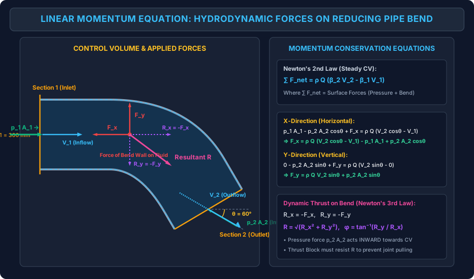
  20. 7.2 Structural Function of a Thrust Block (IS 5330 / AWWA M9)
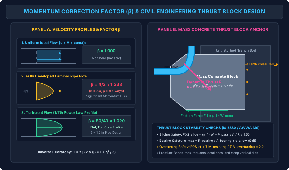
  21. 7.3 Mandatory Geotechnical Stability Checks
  22. 8. Visual Diagrams & Architectural Schematics
  23. 8.1 Hydrodynamic Forces on Pipe Bend Control Volume
  24. 8.2 Momentum Correction Factor (β) & Thrust Block Structural Design
  25. 9. Step-by-Step Numerical Problems with Complete Calculations
  26. Problem 1: Reducing 60° Pipe Bend with Energy Loss & Dynamic Force Resolution
  27. Problem 2: Mathematical Proof & Error Evaluation of Momentum Correction Factor (β)
  28. Problem 3: Design of Mass Concrete Thrust Block at a 90° Pipeline Bend
  29. 10. High-Yield Exam Pitfalls, Traps & Shortcuts
  30. 11. Multi-Exam Question Bank (GATE, ESE, SSC JE, State AE, RRB JE)
  31. Question 1 (GATE CE — Multiple Choice Question)
  32. Question 2 (UPSC ESE Paper-II)
  33. Question 3 (SSC JE)
  34. Question 4 (State PSC AE)
  35. Question 5 (RRB JE)
  36. 12. Comprehensive Summary, Formula Cheatsheet & Academic References
  37. Master Formula Cheatsheet
  38. Academic References & Standard Source Texts

1. Topic Metadata Table

Field Detail
Subject Fluid Mechanics & Hydraulic Machinery (Subject 07)
Chapter Chapter 04: Fluid Dynamics & Momentum Equation
Topic Code FM-04-03
Topic Title Linear Momentum Conservation for a Control Volume, Momentum Correction Factor (β\beta), Hydrodynamic Forces on Pipe Bends, Reducers, Nozzles & Mass Concrete Thrust Block Design
Prerequisites FM-03-02 (Continuity Equation), FM-04-01 (Bernoulli's Theorem & Extended Energy Equation), Vector Mechanics (Newton's 2nd & 3rd Laws of Motion)
Target Examinations GATE CE, UPSC ESE (Paper-II), SSC JE, State PSC AE/JE, RRB JE
Knowledge Level Integral Continuum Mechanics to Applied Municipal Pipeline Structural Anchorage
IS / AWWA / Standard Codes IS 5330 (Criteria for design of anchor blocks for penstocks with expansion joints), IS 12288 (Code of practice for use and laying of ductile iron pipes), AWWA M9 (Concrete Thrust Blocking for Ductile-Iron Pipe), Manual on Water Supply and Treatment (CPHEEO, Ministry of Housing and Urban Affairs)
Key Formulae ∑F⃗net=ρQ(β2V⃗2−β1V⃗1)\sum \vec{F}_{\text{net}} = \rho Q (\beta_2 \vec{V}_2 - \beta_1 \vec{V}_1), β=1AV2∫Au2dA\beta = \frac{1}{A V^2}\int_A u^2 dA, Rx=−FxR_x = -F_x, Ry=−FyR_y = -F_y, R=Rx2+Ry2R = \sqrt{R_x^2 + R_y^2}, Rbend, 90∘=2(pA+ρQV)R_{\text{bend, 90}^\circ} = \sqrt{2}(p A + \rho Q V), FOSslide=μfWblock+PpR≥1.50\text{FOS}_{\text{slide}} = \frac{\mu_f W_{\text{block}} + P_p}{R} \ge 1.50

2. Executive Summary

While Bernoulli's energy equation quantifies scalar mechanical head variations along streamlines, it cannot evaluate vector hydrodynamic reaction forces exerted by moving fluid streams on enclosing physical boundaries. Determining structural anchor requirements, nozzle recoil forces, and bend anchorage in high-pressure conduits requires the Linear Momentum Equation, formulated by applying Newton's second law of motion (∑F⃗=dP⃗dt\sum \vec{F} = \frac{d\vec{P}}{dt}) to a fixed macroscopic Fluid Control Volume (CV) via the Reynolds Transport Theorem.

Under steady, incompressible flow conditions, the net vector force acting on the fluid within a control volume identically equals the net efflux rate of linear momentum across its control surfaces:

∑F⃗net=M⃗˙out−M⃗˙in=∫CS,outV⃗(ρV⃗⋅n^)dA−∫CS,inV⃗(ρV⃗⋅n^)dA\sum \vec{F}_{\text{net}} = \dot{\vec{M}}_{\text{out}} - \dot{\vec{M}}_{\text{in}} = \int_{\text{CS,out}} \vec{V} (\rho \vec{V} \cdot \hat{n}) dA - \int_{\text{CS,in}} \vec{V} (\rho \vec{V} \cdot \hat{n}) dA

Applying the bulk mean velocity V=Q/AV = Q/A across finite conduit cross-sections introduces the Momentum Correction Factor (Boussinesq Coefficient) β=1AV2∫Au2dA\beta = \frac{1}{A V^2}\int_A u^2 dA. For uniform flow, β=1.00\beta = 1.00; for laminar circular pipe flow, β=4/3≈1.33\beta = 4/3 \approx 1.33; and for turbulent pipe flow, β=50/49≈1.02\beta = 50/49 \approx 1.02. Because velocity fluctuations amplify momentum flux less aggressively than kinetic energy flux, the fundamental physical inequality 1.0≤β<α1.0 \le \beta < \alpha holds universally across all real flow fields.

In civil and hydraulic engineering, the primary application of the linear momentum equation is calculating the Dynamic Hydrodynamic Thrust (R⃗\vec{R}) exerted by pressurized water streams on pipe bends, elbows, wyes, reducers, and dead ends:

  • The total force exerted by the fluid on a bend is composed of two interacting components:
    1. Static Pressure Thrust: Resulting from the imbalance of internal hydrostatic/piezometric normal forces (p1A1p_1 A_1 and p2A2p_2 A_2).
    2. Dynamic Momentum Thrust: Resulting from the forced change in direction and magnitude of the fluid momentum vector (ρQ(V⃗1−V⃗2)\rho Q (\vec{V}_1 - \vec{V}_2)).
  • The Critical Directionality Trap: The static pressure force exerted by the downstream pipe on the control volume (p2A2p_2 A_2) acts inward towards the interior of the control volume (opposing outward flow direction). Neglecting this sign inversion is the single most pervasive source of error in competitive examination calculations!
  • Civil Infrastructure Deliverable (Thrust Blocks): In buried water distribution networks and surface penstocks, flexible push-on joints cannot sustain axial tension. The unbonded resultant thrust RR will pull bell-and-spigot joints apart, precipitating catastrophic pipeline rupture and urban flooding. Engineers must size massive Concrete Thrust Blocks designed to anchor the bend securely into undisturbed trench soil, verified against basal sliding (FOS≥1.50\text{FOS} \ge 1.50), soil bearing failure (σ≤qallow\sigma \le q_{\text{allow}}), and overturning (FOS≥2.0\text{FOS} \ge 2.0).

3. Reynolds Transport Theorem & Control Volume Linear Momentum Formulation

3.1 Reynolds Transport Theorem (RTT)

Let BB represent an extensive fluid property (such as total mass mm, linear momentum mV⃗m\vec{V}, or total energy EE), and let βint=dB/dm\beta_{\text{int}} = dB/dm be the corresponding intensive property (property per unit mass). The Reynolds Transport Theorem connects the time rate of change of property BB for a moving material system to variations within a fixed spatial Control Volume (CV) bounded by Control Surface (CS):

dBsysdt=ddt∫CVρβint d∀+∫CSρβint(V⃗r⋅n^)dA\frac{d B_{\text{sys}}}{dt} = \frac{d}{dt}\int_{\text{CV}} \rho \beta_{\text{int}} \, d\forall + \int_{\text{CS}} \rho \beta_{\text{int}} (\vec{V}_r \cdot \hat{n}) dA

where V⃗r\vec{V}_r is the fluid velocity relative to the control surface, and n^\hat{n} is the outward-pointing unit normal vector.

3.2 Application to Linear Momentum

For linear momentum, the extensive property is B⃗=mV⃗\vec{B} = m\vec{V}, so the intensive property is:

βint=d(mV⃗)dm=V⃗\beta_{\text{int}} = \frac{d(m\vec{V})}{dm} = \vec{V}

Newton's second law for the fluid system states:

∑F⃗net=(dP⃗sysdt)\sum \vec{F}_{\text{net}} = \left(\frac{d\vec{P}_{\text{sys}}}{dt}\right)

Substituting into the RTT for a fixed control volume (V⃗r=V⃗\vec{V}_r = \vec{V}):

∑F⃗net=∂∂t∫CVρV⃗ d∀+∫CSρV⃗(V⃗⋅n^)dA\sum \vec{F}_{\text{net}} = \frac{\partial}{\partial t}\int_{\text{CV}} \rho \vec{V} \, d\forall + \int_{\text{CS}} \rho \vec{V} (\vec{V} \cdot \hat{n}) dA

For steady flow (∂/∂t=0\partial/\partial t = 0), the local temporal storage term vanishes:

∑F⃗net=∫CSρV⃗(V⃗⋅n^)dA=∑m˙outV⃗out−∑m˙inV⃗in\sum \vec{F}_{\text{net}} = \int_{\text{CS}} \rho \vec{V} (\vec{V} \cdot \hat{n}) dA = \sum \dot{m}_{\text{out}} \vec{V}_{\text{out}} - \sum \dot{m}_{\text{in}} \vec{V}_{\text{in}}

3.3 Classification of Net Applied Forces (∑F⃗net\sum \vec{F}_{\text{net}})

The net force acting on the fluid within the control volume consists of:

∑F⃗net=F⃗body+F⃗surface\sum \vec{F}_{\text{net}} = \vec{F}_{\text{body}} + \vec{F}_{\text{surface}}
  1. Body Forces (F⃗body\vec{F}_{\text{body}}): Gravitational weight of the fluid enclosed within the control volume (W⃗=∫CVρg⃗ d∀\vec{W} = \int_{\text{CV}} \rho \vec{g} \, d\forall). In horizontal pipe bends, the vertical weight acts along the zz-axis, exerting zero component in the horizontal x–yx\text{--}y plane of motion.
  2. Surface Forces (F⃗surface\vec{F}_{\text{surface}}):
    • Pressure Forces (F⃗p\vec{F}_p): Hydrostatic/piezometric normal forces acting across all open flow boundaries (inlet and outlet planes).
    • Shear and Normal Wall Reaction Forces (F⃗wall\vec{F}_{\text{wall}}): The mechanical force exerted by the solid conduit walls on the fluid control volume (F⃗wall=Fxi^+Fyj^\vec{F}_{\text{wall}} = F_x \hat{i} + F_y \hat{j}).

4. Momentum Correction Factor (β\beta, Boussinesq Coefficient)

In practical 1D engineering analysis, pipe calculations utilize the cross-sectional bulk mean velocity V=Q/AV = Q/A. However, viscous friction at solid boundaries creates non-uniform velocity distributions u(y)u(y) or u(r)u(r). The true rate of momentum flux transmitted across an elemental area dAdA is:

dM˙actual=(dm)u=(ρu dA)u=ρu2 dAd\dot{M}_{\text{actual}} = (dm) u = (\rho u \, dA) u = \rho u^2 \, dA

Integrating over the entire cross section AA, the actual linear momentum flux is:

M˙actual=ρ∫Au2 dA\dot{M}_{\text{actual}} = \rho \int_A u^2 \, dA

If calculated naively using the 1D average velocity VV:

M˙1D=(ρAV)V=ρAV2\dot{M}_{\text{1D}} = (\rho A V) V = \rho A V^2

Because the mean of squares is always greater than or equal to the square of the mean:

1A∫Au2dA≥V2\frac{1}{A}\int_A u^2 dA \ge V^2

The Momentum Correction Factor (Boussinesq Coefficient) β\beta is defined as:

β=M˙actualM˙1D=ρ∫Au2dAρAV2=1AV2∫Au2 dA\beta = \frac{\dot{M}_{\text{actual}}}{\dot{M}_{\text{1D}}} = \frac{\rho \int_A u^2 dA}{\rho A V^2} = \frac{1}{A V^2}\int_A u^2 \, dA

4.1 Analytical Derivation for Fully Developed Laminar Pipe Flow

For laminar flow in a circular pipe of radius RR, the Hagen-Poiseuille parabolic velocity distribution is:

u(r)=Umax⁡[1−(rR)2],V=Umax⁡2u(r) = U_{\max} \left[1 - \left(\frac{r}{R}\right)^2\right], \quad V = \frac{U_{\max}}{2}

Let η=(r/R)2  ⟹  2πrdr=πR2dη\eta = (r/R)^2 \implies 2\pi r dr = \pi R^2 d\eta. Substitute into the definition of β\beta:

β=1πR2(Umax⁡/2)2∫0RUmax⁡2[1−(rR)2]22πrdr\beta = \frac{1}{\pi R^2 (U_{\max}/2)^2} \int_0^R U_{\max}^2 \left[1 - \left(\frac{r}{R}\right)^2\right]^2 2\pi r dr β=4πR2∫01(1−η)2(πR2dη)=4∫01(1−η)2dη\beta = \frac{4}{\pi R^2} \int_0^1 (1 - \eta)^2 (\pi R^2 d\eta) = 4 \int_0^1 (1 - \eta)^2 d\eta

Evaluating the integral:

∫01(1−η)2dη=[−(1−η)33]01=0−(−13)=13\int_0^1 (1 - \eta)^2 d\eta = \left[ -\frac{(1-\eta)^3}{3} \right]_0^1 = 0 - \left(-\frac{1}{3}\right) = \frac{1}{3}

Therefore:

βlaminar, pipe=4×13=43≈1.3333\beta_{\text{laminar, pipe}} = 4 \times \frac{1}{3} = \frac{4}{3} \approx 1.3333

4.2 Analytical Derivation for Turbulent Pipe Flow (1/7th Power Law)

For turbulent pipe flow, the velocity follows Prandtl's 1/7th power law:

uUmax⁡=(1−rR)1/7=ξ1/7,V=4960Umax⁡\frac{u}{U_{\max}} = \left(1 - \frac{r}{R}\right)^{1/7} = \xi^{1/7}, \quad V = \frac{49}{60} U_{\max}

where ξ=y/R=(R−r)/R\xi = y/R = (R - r)/R. Thus r=R(1−ξ)r = R(1 - \xi) and dr=−Rdξdr = -R d\xi. The momentum flux integral is:

∫Au2dA=2πUmax⁡2∫0R(yR)2/7(R−y)dy=2πR2Umax⁡2∫01ξ2/7(1−ξ)dξ\int_A u^2 dA = 2\pi U_{\max}^2 \int_0^R \left(\frac{y}{R}\right)^{2/7} (R - y) dy = 2\pi R^2 U_{\max}^2 \int_0^1 \xi^{2/7} (1 - \xi) d\xi ∫01(ξ2/7−ξ9/7)dξ=79−716=112−63144=49144\int_0^1 (\xi^{2/7} - \xi^{9/7}) d\xi = \frac{7}{9} - \frac{7}{16} = \frac{112 - 63}{144} = \frac{49}{144} ∫Au2dA=2πR2Umax⁡2(49144)\int_A u^2 dA = 2\pi R^2 U_{\max}^2 \left(\frac{49}{144}\right)

Now compute β\beta:

β=∫Au2dAAV2=2πR2Umax⁡2(49/144)πR2(4960Umax⁡)2=2×4914424013600=98144×36002401=98×252401=24502401=5049≈1.0204\beta = \frac{\int_A u^2 dA}{A V^2} = \frac{2\pi R^2 U_{\max}^2 (49/144)}{\pi R^2 \left(\frac{49}{60} U_{\max}\right)^2} = \frac{2 \times \frac{49}{144}}{\frac{2401}{3600}} = \frac{98}{144} \times \frac{3600}{2401} = \frac{98 \times 25}{2401} = \frac{2450}{2401} = \frac{50}{49} \approx 1.0204
Flow Regime Velocity Profile β\beta (Momentum Factor) α\alpha (Kinetic Energy Factor) Relationship
Uniform Ideal Flow u=V=constu = V = \text{const} β=1.000\beta = 1.000 α=1.000\alpha = 1.000 α=β=1\alpha = \beta = 1
Laminar Flow (Circular Pipe) Parabolic u=Umax⁡[1−(r/R)2]u = U_{\max}[1-(r/R)^2] β=4/3≈1.333\beta = 4/3 \approx 1.333 α=2.000\alpha = 2.000 β<α\beta < \alpha
Laminar Flow (Parallel Plates) Parabolic 2D β=6/5=1.200\beta = 6/5 = 1.200 α=54/35≈1.543\alpha = 54/35 \approx 1.543 β<α\beta < \alpha
Turbulent Pipe Flow 1/7th Power Law β=50/49≈1.020\beta = 50/49 \approx 1.020 α≈1.058\alpha \approx 1.058 β<α\beta < \alpha
Turbulent Boundary Layer Logarithmic Profile β≈1.01–1.03\beta \approx 1.01\text{--}1.03 α≈1.03–1.06\alpha \approx 1.03\text{--}1.06 β≈1.0\beta \approx 1.0

Universal Inequality (GATE CE): For any real non-uniform velocity distribution:

1.0≤β<α1.0 \le \beta < \alpha

(If the velocity profile is expressed as u=V(1+η)u = V(1 + \eta) where ∫ηdA=0\int \eta dA = 0, then to second-order approximation: β≈1+η2‾\beta \approx 1 + \overline{\eta^2} and α≈1+3η2‾  ⟹  α−1≈3(β−1)\alpha \approx 1 + 3\overline{\eta^2} \implies \alpha - 1 \approx 3(\beta - 1)).


5. Dynamic Hydrodynamic Forces on Reducing Pipe Bends & Reducers

Consider a horizontal reducing pipe bend deflecting steady water flow through an angle θ\theta in the x–yx\text{--}y plane.

  • Section 1 (Inlet): Area A1A_1, internal gauge pressure p1p_1, velocity V1V_1 directed along the +x+x axis.
  • Section 2 (Outlet): Area A2A_2, internal gauge pressure p2p_2, velocity V2V_2 directed at angle θ\theta to the +x+x axis.
                         ^ y
                         |           Section 2 (Outlet)
                         |             /
                         |            /  A2, p2, V2 at angle theta
                         |           +---
                         |          /
                         |         /  Bend Wall Reaction (Fx, Fy)
       p1*A1             |        /
      ======> [Section 1]+-------+-----------------------> x
         A1, p1, V1

5.1 X-Direction Momentum Conservation

Forces acting on the fluid control volume in the xx-direction:

  1. Pressure force at inlet: +p1A1+p_1 A_1 (acts in +x+x direction),
  2. Pressure force at outlet: −p2A2cos⁡θ-p_2 A_2 \cos\theta (acts inward, opposing +x+x),
  3. Component of force exerted by the solid bend wall on the fluid: +Fx+F_x.

Net external force in xx:

∑Fx=p1A1−p2A2cos⁡θ+Fx\sum F_x = p_1 A_1 - p_2 A_2 \cos\theta + F_x

Net momentum efflux rate in xx:

ΔM˙x=m˙(β2V2x−β1V1x)=ρQ(β2V2cos⁡θ−β1V1)\Delta \dot{M}_x = \dot{m} (\beta_2 V_{2x} - \beta_1 V_{1x}) = \rho Q (\beta_2 V_2 \cos\theta - \beta_1 V_1)

Equating:

p1A1−p2A2cos⁡θ+Fx=ρQ(β2V2cos⁡θ−β1V1)p_1 A_1 - p_2 A_2 \cos\theta + F_x = \rho Q (\beta_2 V_2 \cos\theta - \beta_1 V_1)

Solving for the force exerted by the wall on the fluid:

Fx=ρQ(β2V2cos⁡θ−β1V1)−p1A1+p2A2cos⁡θF_x = \rho Q (\beta_2 V_2 \cos\theta - \beta_1 V_1) - p_1 A_1 + p_2 A_2 \cos\theta

5.2 Y-Direction Momentum Conservation

Forces acting on the fluid control volume in the yy-direction:

  1. Pressure force at inlet: 00 (flow is purely along xx),
  2. Pressure force at outlet: −p2A2sin⁡θ-p_2 A_2 \sin\theta (acts inward, opposing +y+y),
  3. Component of force exerted by the solid bend wall on the fluid: +Fy+F_y.

Net external force in yy:

∑Fy=0−p2A2sin⁡θ+Fy\sum F_y = 0 - p_2 A_2 \sin\theta + F_y

Net momentum efflux rate in yy:

ΔM˙y=m˙(β2V2y−β1V1y)=ρQ(β2V2sin⁡θ−0)\Delta \dot{M}_y = \dot{m} (\beta_2 V_{2y} - \beta_1 V_{1y}) = \rho Q (\beta_2 V_2 \sin\theta - 0)

Equating:

−p2A2sin⁡θ+Fy=ρQβ2V2sin⁡θ-p_2 A_2 \sin\theta + F_y = \rho Q \beta_2 V_2 \sin\theta

Solving for the wall reaction force:

Fy=ρQβ2V2sin⁡θ+p2A2sin⁡θ=(ρQβ2V2+p2A2)sin⁡θF_y = \rho Q \beta_2 V_2 \sin\theta + p_2 A_2 \sin\theta = (\rho Q \beta_2 V_2 + p_2 A_2)\sin\theta

5.3 Force Exerted by Fluid on the Pipe Bend (Newton's Third Law)

By Newton's third law of action and reaction, the force R⃗\vec{R} exerted by the moving fluid stream on the pipe bend is equal in magnitude and opposite in direction to the force F⃗\vec{F} exerted by the bend on the fluid:

Rx=−Fx=p1A1−p2A2cos⁡θ−ρQ(β2V2cos⁡θ−β1V1)R_x = -F_x = p_1 A_1 - p_2 A_2 \cos\theta - \rho Q (\beta_2 V_2 \cos\theta - \beta_1 V_1) Ry=−Fy=−(ρQβ2V2+p2A2)sin⁡θR_y = -F_y = -(\rho Q \beta_2 V_2 + p_2 A_2)\sin\theta

The resultant hydrodynamic thrust magnitude RR and its angle of action ϕ\phi relative to the +x+x axis are:

R=Rx2+Ry2R = \sqrt{R_x^2 + R_y^2} ϕ=tan⁡−1(RyRx)\phi = \tan^{-1}\left(\frac{R_y}{R_x}\right)

5.4 Special Case: Constant-Diameter Bend (D1=D2=D,A1=A2=A,V1=V2=VD_1 = D_2 = D, A_1 = A_2 = A, V_1 = V_2 = V)

If head loss is neglected (p1=p2=pp_1 = p_2 = p), and taking β1=β2=1\beta_1 = \beta_2 = 1:

Rx=(pA+ρQV)(1−cos⁡θ)R_x = (p A + \rho Q V)(1 - \cos\theta) Ry=−(pA+ρQV)sin⁡θR_y = -(p A + \rho Q V)\sin\theta

The resultant thrust simplifies analytically to:

R=Rx2+Ry2=(pA+ρQV)(1−cos⁡θ)2+sin⁡2θ=(pA+ρQV)2(1−cos⁡θ)R = \sqrt{R_x^2 + R_y^2} = (p A + \rho Q V) \sqrt{(1 - \cos\theta)^2 + \sin^2\theta} = (p A + \rho Q V) \sqrt{2(1 - \cos\theta)}

Using the half-angle trigonometric identity 2(1−cos⁡θ)=2sin⁡(θ/2)\sqrt{2(1 - \cos\theta)} = 2 \sin(\theta/2):

R=2(pA+ρQV)sin⁡(θ2)R = 2 (p A + \rho Q V) \sin\left(\frac{\theta}{2}\right)

The resultant thrust acts along the external angle bisector:

ϕ=−(180∘−θ2)\phi = -\left(\frac{180^\circ - \theta}{2}\right)
Bend Deflection Angle (θ\theta) Resultant Thrust Formula RR Angle of Action (ϕ\phi)
45∘45^\circ Bend R=2(pA+ρQV)sin⁡22.5∘≈0.765(pA+ρQV)R = 2 (p A + \rho Q V) \sin 22.5^\circ \approx 0.765 (p A + \rho Q V) −67.5∘-67.5^\circ
90∘90^\circ Standard Elbow R=2(pA+ρQV)≈1.414(pA+ρQV)R = \sqrt{2} (p A + \rho Q V) \approx 1.414 (p A + \rho Q V) −45.0∘-45.0^\circ
180∘180^\circ U-Bend / Return Bend R=2(pA+ρQV)R = 2 (p A + \rho Q V) 0∘0^\circ (Direct axial pull)

6. Static Pressure vs Dynamic Momentum Thrust: The Directionality Trap

In competitive examinations and field engineering calculations, catastrophic errors frequently occur due to conceptual misunderstanding of pressure force vectors:

1. Pressure Acts INWARD on the Control Volume

  • Pressure is a compressive normal stress. It always pushes into a surface.
  • At inlet Section 1, the upstream fluid pushes into the control volume: +p1A1i^+p_1 A_1 \hat{i}.
  • At outlet Section 2, the downstream fluid pushes back into the control volume against the outward flow: F⃗p2=−p2A2n^2\vec{F}_{p2} = -p_2 A_2 \hat{n}_2.
  • Common Mistake: Students mistakenly write +p2A2+p_2 A_2 because flow is leaving the control volume. Remember: Flow direction does not alter the fact that fluid pressure is compressive!

2. Relative Magnitude of Static vs Dynamic Thrust

In typical civil water distribution mains (p∼400–800 kPa,V∼1.5–3.0 m/sp \sim 400\text{--}800\text{ kPa}, V \sim 1.5\text{--}3.0\text{ m/s}):

Static Pressure Force Fp=pA=(500×103)×π4(0.40)2≈62.8 kN\text{Static Pressure Force } F_p = p A = (500 \times 10^3) \times \frac{\pi}{4}(0.40)^2 \approx 62.8\text{ kN} Dynamic Momentum Force Fm=ρQV=ρAV2=1000×π4(0.40)2×(2.78)2≈0.97 kN\text{Dynamic Momentum Force } F_m = \rho Q V = \rho A V^2 = 1000 \times \frac{\pi}{4}(0.40)^2 \times (2.78)^2 \approx 0.97\text{ kN} FpFm=62.80.97≈65:1\frac{F_p}{F_m} = \frac{62.8}{0.97} \approx 65 : 1

In high-pressure civil conduits, Static Pressure Thrust dominates dynamic momentum thrust by a factor of 50 to 100! However, during transient water hammer surges or in high-velocity impulse turbines (V∼100 m/sV \sim 100\text{ m/s}), dynamic momentum thrust becomes dominant.


7. Civil Engineering Application: Mass Concrete Thrust Block Design

7.1 The Physical Vulnerability of Buried Pipeline Joints

Modern municipal water supply systems use Ductile Iron (DI), Prestressed Concrete Cylinder Pipes (PCCP), or HDPE pipes joined using flexible push-on rubber gasket joints (e.g., Tyton joints).

  • These joints provide watertight seals under internal hydrostatic pressure while accommodating ground settlement and thermal expansion.
  • However, flexible push-on joints possess zero tensile restraint capacity.
  • When pressurized water encounters a bend, tee, or reducer, the resultant hydrodynamic thrust RR attempts to push the fitting off the pipe barrel. Without external anchorage, the joint pulls apart instantly.

7.2 Structural Function of a Thrust Block (IS 5330 / AWWA M9)

A Thrust Block is an in-situ cast mass concrete block (typically M15 or M20 grade plain concrete) placed between the pipe fitting and the undisturbed vertical trench wall:

  1. It transfers the resultant thrust RR across a wide contact surface area to the native soil.
  2. It mobilizes the passive earth resistance of the undisturbed trench embankment.
  3. Its self-weight generates basal friction along the trench floor.
       Plan View (Looking Down):
                         Pipe Line
                            ||
                            ||
                            ||   Resultant Thrust R
                        ====++=======>  [ Mass Concrete ] ===> Passive Soil
                       /    ||             [ Thrust Block ]       Resistance
                      /     ||                 Weight W
               Pipe  /

7.3 Mandatory Geotechnical Stability Checks

  1. Sliding Stability Check: FOSslide=μfWblock+PpassiveR≥1.50\text{FOS}_{\text{slide}} = \frac{\mu_f W_{\text{block}} + P_{\text{passive}}}{R} \ge 1.50 where:
    • μf\mu_f: Coefficient of friction between cast-in-place concrete and soil floor (μf≈0.35–0.45\mu_f \approx 0.35\text{--}0.45 for sand/gravel, 0.25–0.300.25\text{--}0.30 for clay).
    • Wblock=γconc×∀blockW_{\text{block}} = \gamma_{\text{conc}} \times \forall_{\text{block}}: Total gravitational weight of the mass concrete block (γconc≈24.0 kN/m3\gamma_{\text{conc}} \approx 24.0\text{ kN/m}^3).
    • PpassiveP_{\text{passive}}: Total passive earth pressure developed against the trench wall.
  2. Soil Bearing Capacity Check: The thrust force per unit contact area against the trench soil must not exceed the allowable passive soil bearing capacity: σ=RAbearing≤qallow, soil\sigma = \frac{R}{A_{\text{bearing}}} \le q_{\text{allow, soil}}   ⟹  Abearing, min=Rqallow, soil\implies A_{\text{bearing, min}} = \frac{R}{q_{\text{allow, soil}}} (Typical safe bearing capacities: Soft clay: 50 kPa50\text{ kPa}; Stiff clay: 100 kPa100\text{ kPa}; Compact sand: 150 kPa150\text{ kPa}; Dense gravel: 250 kPa250\text{ kPa}; Solid rock: >500 kPa> 500\text{ kPa}).
  3. Overturning Stability Check: FOSoverturning=∑Mresisting∑Moverturning≥2.0\text{FOS}_{\text{overturning}} = \frac{\sum M_{\text{resisting}}}{\sum M_{\text{overturning}}} \ge 2.0

8. Visual Diagrams & Architectural Schematics

8.1 Hydrodynamic Forces on Pipe Bend Control Volume

The schematic below presents the complete vector control volume force resolution on an inclined reducing pipe bend, detailing inlet/outlet pressure vectors, fluid momentum fluxes, wall reaction forces, and the resultant thrust vector.

Hydrodynamic Forces on Reducing Pipe Bend Control Volume

8.2 Momentum Correction Factor (β\beta) & Thrust Block Structural Design

The multi-panel diagram below contrasts velocity profile shapes and their corresponding β\beta factors against the geotechnical stability mechanics of a civil mass concrete thrust block anchor.

Thrust Block Design and Momentum Factor Profiles

9. Step-by-Step Numerical Problems with Complete Calculations

Problem 1: Reducing 60° Pipe Bend with Energy Loss & Dynamic Force Resolution

Problem Statement: A horizontal reducing pipe bend deflects a steady water stream (ρ=1000 kg/m3,γ=9810 N/m3\rho = 1000\text{ kg/m}^3, \gamma = 9810\text{ N/m}^3) through a deflection angle θ=60∘\theta = 60^\circ.

  • Inlet diameter: D1=300 mm=0.30 mD_1 = 300\text{ mm} = 0.30\text{ m}.
  • Outlet diameter: D2=150 mm=0.15 mD_2 = 150\text{ mm} = 0.15\text{ m}.
  • Volumetric flow rate: Q=0.250 m3/sQ = 0.250\text{ m}^3/\text{s} (250 L/s250\text{ L/s}).
  • Pressure at inlet: p1=300 kPa=300×103 N/m2p_1 = 300\text{ kPa} = 300 \times 10^3\text{ N/m}^2.
  • Head loss through the bend is given as hL=0.40V222gh_L = 0.40 \frac{V_2^2}{2g}.
  • Assume uniform velocity profiles at inlet and outlet (β1=β2=1.0\beta_1 = \beta_2 = 1.0).
  • Take g=9.81 m/s2g = 9.81\text{ m/s}^2.

Determine:

  1. Flow velocities V1V_1 and V2V_2 and their velocity heads,
  2. Head loss hLh_L and static pressure p2p_2 at the outlet,
  3. Force components Fx,FyF_x, F_y exerted by the bend wall on the water,
  4. Resultant force RR exerted by the water on the bend and its inclination ϕ\phi to the +x+x axis.

Solution & Step-by-Step Calculation:

Step 1: Compute cross-sectional areas and flow velocities

A1=π4D12=π4(0.30)2=0.0706858 m2A_1 = \frac{\pi}{4} D_1^2 = \frac{\pi}{4} (0.30)^2 = 0.0706858\text{ m}^2 A2=π4D22=π4(0.15)2=0.0176715 m2A_2 = \frac{\pi}{4} D_2^2 = \frac{\pi}{4} (0.15)^2 = 0.0176715\text{ m}^2 V1=QA1=0.2500.0706858=3.53678 m/s≈3.537 m/sV_1 = \frac{Q}{A_1} = \frac{0.250}{0.0706858} = 3.53678\text{ m/s} \approx 3.537\text{ m/s} V2=QA2=0.2500.0176715=14.14711 m/s≈14.147 m/sV_2 = \frac{Q}{A_2} = \frac{0.250}{0.0176715} = 14.14711\text{ m/s} \approx 14.147\text{ m/s}

Velocity heads:

V122g=(3.53678)22×9.81=12.508819.62=0.63755 m\frac{V_1^2}{2g} = \frac{(3.53678)^2}{2 \times 9.81} = \frac{12.5088}{19.62} = 0.63755\text{ m} V222g=(14.14711)22×9.81=200.140719.62=10.20085 m\frac{V_2^2}{2g} = \frac{(14.14711)^2}{2 \times 9.81} = \frac{200.1407}{19.62} = 10.20085\text{ m}

Head loss in bend:

hL=0.40×V222g=0.40×10.20085=4.08034 mh_L = 0.40 \times \frac{V_2^2}{2g} = 0.40 \times 10.20085 = 4.08034\text{ m}

Step 2: Compute outlet pressure p2p_2 using extended Bernoulli equation Horizontal bend   ⟹  z1=z2\implies z_1 = z_2.

p1γ+V122g=p2γ+V222g+hL\frac{p_1}{\gamma} + \frac{V_1^2}{2g} = \frac{p_2}{\gamma} + \frac{V_2^2}{2g} + h_L p1γ=300×103 N/m29810 N/m3=30.58104 m\frac{p_1}{\gamma} = \frac{300 \times 10^3\text{ N/m}^2}{9810\text{ N/m}^3} = 30.58104\text{ m} p2γ=p1γ+V122g−V222g−hL\frac{p_2}{\gamma} = \frac{p_1}{\gamma} + \frac{V_1^2}{2g} - \frac{V_2^2}{2g} - h_L p2γ=30.58104+0.63755−10.20085−4.08034=16.93740 m\frac{p_2}{\gamma} = 30.58104 + 0.63755 - 10.20085 - 4.08034 = 16.93740\text{ m} p2=16.93740 m×9810 N/m3=166,155.9 Pa≈166.16 kPap_2 = 16.93740\text{ m} \times 9810\text{ N/m}^3 = 166,155.9\text{ Pa} \approx 166.16\text{ kPa}

Step 3: Linear Momentum Equation in X-Direction

∑Fx=p1A1−p2A2cos⁡60∘+Fx=ρQ(V2cos⁡60∘−V1)\sum F_x = p_1 A_1 - p_2 A_2 \cos 60^\circ + F_x = \rho Q (V_2 \cos 60^\circ - V_1)

Compute individual terms:

p1A1=300,000×0.0706858=21,205.75 Np_1 A_1 = 300,000 \times 0.0706858 = 21,205.75\text{ N} p2A2cos⁡60∘=166,155.9×0.0176715×0.50=2,936.22×0.50=1,468.11 Np_2 A_2 \cos 60^\circ = 166,155.9 \times 0.0176715 \times 0.50 = 2,936.22 \times 0.50 = 1,468.11\text{ N} Pressure term (p1A1−p2A2cos⁡60∘)=21,205.75−1,468.11=19,737.64 N\text{Pressure term } (p_1 A_1 - p_2 A_2 \cos 60^\circ) = 21,205.75 - 1,468.11 = 19,737.64\text{ N} Momentum term ρQ(V2cos⁡60∘−V1)=1000×0.250×(14.14711×0.50−3.53678)\text{Momentum term } \rho Q (V_2 \cos 60^\circ - V_1) = 1000 \times 0.250 \times (14.14711 \times 0.50 - 3.53678) =250×(7.07355−3.53678)=250×3.53678=884.19 N= 250 \times (7.07355 - 3.53678) = 250 \times 3.53678 = 884.19\text{ N}

Solving for FxF_x:

19,737.64+Fx=884.19  ⟹  Fx=884.19−19,737.64=−18,853.45 N19,737.64 + F_x = 884.19 \implies F_x = 884.19 - 19,737.64 = -18,853.45\text{ N}

Step 4: Linear Momentum Equation in Y-Direction

∑Fy=0−p2A2sin⁡60∘+Fy=ρQ(V2sin⁡60∘−0)\sum F_y = 0 - p_2 A_2 \sin 60^\circ + F_y = \rho Q (V_2 \sin 60^\circ - 0)

Compute individual terms:

sin⁡60∘=0.866025\sin 60^\circ = 0.866025 p2A2sin⁡60∘=2,936.22×0.866025=2,542.84 Np_2 A_2 \sin 60^\circ = 2,936.22 \times 0.866025 = 2,542.84\text{ N} ρQV2sin⁡60∘=1000×0.250×14.14711×0.866025=250×12.25175=3,062.94 N\rho Q V_2 \sin 60^\circ = 1000 \times 0.250 \times 14.14711 \times 0.866025 = 250 \times 12.25175 = 3,062.94\text{ N}

Solving for FyF_y:

−2,542.84+Fy=3,062.94  ⟹  Fy=3,062.94+2,542.84=5,605.78 N-2,542.84 + F_y = 3,062.94 \implies F_y = 3,062.94 + 2,542.84 = 5,605.78\text{ N}

Step 5: Force Exerted by Water on the Bend (R⃗\vec{R}) By Newton's third law:

Rx=−Fx=−(−18,853.45 N)=+18,853.45 N=+18.853 kNR_x = -F_x = -(-18,853.45\text{ N}) = +18,853.45\text{ N} = +18.853\text{ kN} Ry=−Fy=−(+5,605.78 N)=−5,605.78 N=−5.606 kNR_y = -F_y = -(+5,605.78\text{ N}) = -5,605.78\text{ N} = -5.606\text{ kN}

Resultant magnitude and direction:

R=Rx2+Ry2=(18,853.45)2+(−5,605.78)2=355,452,476+31,424,769=386,877,245=19,669.19 N≈19.669 kNR = \sqrt{R_x^2 + R_y^2} = \sqrt{(18,853.45)^2 + (-5,605.78)^2} = \sqrt{355,452,476 + 31,424,769} = \sqrt{386,877,245} = 19,669.19\text{ N} \approx 19.669\text{ kN} ϕ=tan⁡−1(RyRx)=tan⁡−1(−5,605.7818,853.45)=tan⁡−1(−0.29733)=−16.56∘\phi = \tan^{-1}\left(\frac{R_y}{R_x}\right) = \tan^{-1}\left(\frac{-5,605.78}{18,853.45}\right) = \tan^{-1}(-0.29733) = -16.56^\circ

(The resultant thrust is 19.67 kN19.67\text{ kN} directed at 16.56∘16.56^\circ below the horizontal +x+x axis).


Problem 2: Mathematical Proof & Error Evaluation of Momentum Correction Factor (β\beta)

Problem Statement:

  1. Derive from first principles that β=4/3\beta = 4/3 for laminar flow in a circular conduit having velocity distribution u(r)=U0[1−(r/R)2]u(r) = U_0 [1 - (r/R)^2].
  2. Derive that β=50/49≈1.0204\beta = 50/49 \approx 1.0204 for turbulent flow obeying the 1/7th power law u(r)=U0(1−r/R)1/7u(r) = U_0 (1 - r/R)^{1/7}.
  3. In a dredging slurry pipeline conveying dense sediment-water mixture (ρ=1350 kg/m3\rho = 1350\text{ kg/m}^3) under laminar conditions with volumetric discharge Q=0.080 m3/sQ = 0.080\text{ m}^3/\text{s} through pipe diameter D=200 mmD = 200\text{ mm}, compute the true dynamic momentum flux in N\text{N}. Calculate the percentage error if an engineer naively neglects β\beta by setting β=1.0\beta = 1.0.

Solution & Step-by-Step Calculation:

Step 1: Proof for Laminar Flow Mean velocity V=U0/2V = U_0/2.

β=1πR2V2∫0Ru2(r)⋅2πrdr=2πU02πR2(U0/2)2∫0R[1−(rR)2]2rdr\beta = \frac{1}{\pi R^2 V^2}\int_0^R u^2(r) \cdot 2\pi r dr = \frac{2\pi U_0^2}{\pi R^2 (U_0/2)^2} \int_0^R \left[1 - \left(\frac{r}{R}\right)^2\right]^2 r dr

Let w=(r/R)2  ⟹  rdr=R22dww = (r/R)^2 \implies r dr = \frac{R^2}{2} dw:

β=8R2∫01(1−w)2(R22dw)=4∫01(1−2w+w2)dw=4[w−w2+w33]01=4(1−1+13)=43≈1.3333\beta = \frac{8}{R^2} \int_0^1 (1 - w)^2 \left(\frac{R^2}{2} dw\right) = 4 \int_0^1 (1 - 2w + w^2) dw = 4 \left[ w - w^2 + \frac{w^3}{3} \right]_0^1 = 4 \left( 1 - 1 + \frac{1}{3} \right) = \frac{4}{3} \approx 1.3333

Step 2: Proof for Turbulent 1/7th Power Law Let ξ=y/R=1−r/R\xi = y/R = 1 - r/R.

V=4960U0V = \frac{49}{60} U_0 ∫Au2dA=2πR2U02∫01ξ2/7(1−ξ)dξ=2πR2U02(79−716)=2πR2U02(49144)\int_A u^2 dA = 2\pi R^2 U_0^2 \int_0^1 \xi^{2/7} (1 - \xi) d\xi = 2\pi R^2 U_0^2 \left(\frac{7}{9} - \frac{7}{16}\right) = 2\pi R^2 U_0^2 \left(\frac{49}{144}\right)

Substitute into β=∫u2dAAV2\beta = \frac{\int u^2 dA}{A V^2}:

β=2πR2U02(49/144)πR2(4960U0)2=2×49144(4960)2=98144×36002401=24502401=5049≈1.0204\beta = \frac{2\pi R^2 U_0^2 (49/144)}{\pi R^2 \left(\frac{49}{60} U_0\right)^2} = \frac{2 \times \frac{49}{144}}{\left(\frac{49}{60}\right)^2} = \frac{98}{144} \times \frac{3600}{2401} = \frac{2450}{2401} = \frac{50}{49} \approx 1.0204

Step 3: Slurry Pipeline True Momentum Flux and Error

A=π4(0.20)2=0.0314159 m2A = \frac{\pi}{4}(0.20)^2 = 0.0314159\text{ m}^2 V=QA=0.0800.0314159=2.54648 m/sV = \frac{Q}{A} = \frac{0.080}{0.0314159} = 2.54648\text{ m/s} Nominal Momentum Flux (assuming β=1.0)=M˙1D=ρQV=1350×0.080×2.54648=275.02 N\text{Nominal Momentum Flux (assuming } \beta = 1.0) = \dot{M}_{\text{1D}} = \rho Q V = 1350 \times 0.080 \times 2.54648 = 275.02\text{ N} True Momentum Flux=M˙true=βρQV=43×275.02 N=366.69 N\text{True Momentum Flux} = \dot{M}_{\text{true}} = \beta \rho Q V = \frac{4}{3} \times 275.02\text{ N} = 366.69\text{ N} Percentage Underestimation Error=True−NominalTrue×100%=4/3−1.04/3×100%=1/34/3×100%=25.0%\text{Percentage Underestimation Error} = \frac{\text{True} - \text{Nominal}}{\text{True}} \times 100\% = \frac{4/3 - 1.0}{4/3} \times 100\% = \frac{1/3}{4/3} \times 100\% = 25.0\%

(Neglecting β\beta in laminar flow underpredicts dynamic momentum thrust by exactly 25%).


Problem 3: Design of Mass Concrete Thrust Block at a 90° Pipeline Bend

Problem Statement: A ductile iron municipal water transmission pipeline of diameter D=400 mm=0.40 mD = 400\text{ mm} = 0.40\text{ m} carries water under steady flow at volumetric discharge Q=0.350 m3/sQ = 0.350\text{ m}^3/\text{s} and internal working gauge pressure p=500 kPa=500×103 N/m2p = 500\text{ kPa} = 500 \times 10^3\text{ N/m}^2.

  1. At a horizontal 90∘90^\circ elbow (θ=90∘\theta = 90^\circ), compute the static pressure force FpF_p, dynamic momentum force FmF_m, and the total resultant hydrodynamic thrust RR exerted by the water on the bend.
  2. To anchor the elbow, a mass concrete thrust block (γconc=24.0 kN/m3\gamma_{\text{conc}} = 24.0\text{ kN/m}^3) is cast against undisturbed trench soil. The allowable passive soil bearing capacity is qallow=150 kPaq_{\text{allow}} = 150\text{ kPa}, and the coefficient of friction between the concrete block base and the trench floor is μf=0.45\mu_f = 0.45.
  3. Neglecting passive soil resistance on the sides and relying purely on base friction with a factor of safety FOSslide=1.50\text{FOS}_{\text{slide}} = 1.50, determine the required mass of concrete and concrete volume in m3\text{m}^3.
  4. Determine the minimum contact bearing area AbearingA_{\text{bearing}} required against the trench soil.

Solution & Step-by-Step Calculation:

Step 1: Compute Flow Velocity, Cross-Sectional Area, and Forces

A=π4D2=π4(0.40)2=0.125664 m2A = \frac{\pi}{4} D^2 = \frac{\pi}{4} (0.40)^2 = 0.125664\text{ m}^2 V=QA=0.3500.125664=2.78521 m/sV = \frac{Q}{A} = \frac{0.350}{0.125664} = 2.78521\text{ m/s}

Static pressure force:

Fp=pA=500×103 N/m2×0.125664 m2=62,831.85 N=62.83 kNF_p = p A = 500 \times 10^3\text{ N/m}^2 \times 0.125664\text{ m}^2 = 62,831.85\text{ N} = 62.83\text{ kN}

Dynamic momentum force:

Fm=ρQV=1000×0.350×2.78521=974.82 N=0.975 kNF_m = \rho Q V = 1000 \times 0.350 \times 2.78521 = 974.82\text{ N} = 0.975\text{ kN}

Step 2: Resultant Hydrodynamic Thrust on the 90° Bend For a symmetrical 90∘90^\circ bend (A1=A2,V1=V2A_1 = A_2, V_1 = V_2):

Rx=Fp+Fm=62,831.85+974.82=63,806.67 N=63.81 kNR_x = F_p + F_m = 62,831.85 + 974.82 = 63,806.67\text{ N} = 63.81\text{ kN} Ry=−(Fp+Fm)=−63,806.67 N=−63.81 kNR_y = -(F_p + F_m) = -63,806.67\text{ N} = -63.81\text{ kN} R=Rx2+Ry2=2×(Fp+Fm)=1.414214×63,806.67 N=90,236.2 N≈90.24 kNR = \sqrt{R_x^2 + R_y^2} = \sqrt{2} \times (F_p + F_m) = 1.414214 \times 63,806.67\text{ N} = 90,236.2\text{ N} \approx 90.24\text{ kN}

Directed at ϕ=−45.0∘\phi = -45.0^\circ (along the external angle bisector).

Step 3: Minimum Concrete Volume for Sliding Safety (FOSslide=1.50\text{FOS}_{\text{slide}} = 1.50)

FOSslide=μfWblockR≥1.50\text{FOS}_{\text{slide}} = \frac{\mu_f W_{\text{block}}}{R} \ge 1.50 Wreq=1.50×Rμf=1.50×90,236.2 N0.45=135,354.30.45=300,787 N=300.79 kNW_{\text{req}} = \frac{1.50 \times R}{\mu_f} = \frac{1.50 \times 90,236.2\text{ N}}{0.45} = \frac{135,354.3}{0.45} = 300,787\text{ N} = 300.79\text{ kN}

Concrete weight density: γconc=24.0 kN/m3=24,000 N/m3\gamma_{\text{conc}} = 24.0\text{ kN/m}^3 = 24,000\text{ N/m}^3. Required volume of mass concrete:

∀block=Wreqγconc=300,787 N24,000 N/m3=12.5328 m3≈12.53 m3\forall_{\text{block}} = \frac{W_{\text{req}}}{\gamma_{\text{conc}}} = \frac{300,787\text{ N}}{24,000\text{ N/m}^3} = 12.5328\text{ m}^3 \approx 12.53\text{ m}^3

Step 4: Required Soil Contact Bearing Area The resultant thrust R=90.24 kNR = 90.24\text{ kN} must be transferred safely to the native trench wall without exceeding the allowable soil bearing capacity qallow=150 kPaq_{\text{allow}} = 150\text{ kPa}:

Abearing≥R×FOSbearingqallowA_{\text{bearing}} \ge \frac{R \times \text{FOS}_{\text{bearing}}}{q_{\text{allow}}}

Using working allowable stress design where factor of safety is inherent in qallowq_{\text{allow}}:

Abearing=Rqallow=90.236 kN150 kN/m2=0.6016 m2A_{\text{bearing}} = \frac{R}{q_{\text{allow}}} = \frac{90.236\text{ kN}}{150\text{ kN/m}^2} = 0.6016\text{ m}^2

If applying an explicit engineering factor of safety FOS=1.50\text{FOS} = 1.50:

Abearing, safe=1.50×90.236150=0.9024 m2≈0.90 m2A_{\text{bearing, safe}} = \frac{1.50 \times 90.236}{150} = 0.9024\text{ m}^2 \approx 0.90\text{ m}^2

(Design Specification: Cast a concrete block of dimensions 2.5 m (length)×2.5 m (width)×2.0 m (depth)=12.5 m32.5\text{ m (length)} \times 2.5\text{ m (width)} \times 2.0\text{ m (depth)} = 12.5\text{ m}^3, providing a vertical bearing face of 2.5 m×2.0 m=5.0 m2≫0.90 m22.5\text{ m} \times 2.0\text{ m} = 5.0\text{ m}^2 \gg 0.90\text{ m}^2, guaranteeing complete structural stability).


10. High-Yield Exam Pitfalls, Traps & Shortcuts

  1. The Outlet Pressure Direction Trap (p2A2p_2 A_2 Acts Inward):

    • Trap: Writing the xx-force balance as ∑Fx=p1A1+p2A2cos⁡θ+Fx\sum F_x = p_1 A_1 + p_2 A_2 \cos\theta + F_x.
    • Truth: Fluid pressure is always compressive. It pushes inward into the control volume; therefore, at the outlet, its component along +x+x is −p2A2cos⁡θ-p_2 A_2 \cos\theta.
  2. The "Dynamic Force Equals Pressure Force" Fallacy:

    • Trap: Neglecting pAp A and using only ρQΔV\rho Q \Delta V for the force on a pipe bend.
    • Truth: In closed-conduit water mains, the static pressure force pAp A is often 50 to 100 times larger than the dynamic momentum force ρQV\rho Q V. Never omit pAp A unless the problem explicitly states that the pipe discharges freely into the atmosphere (p=0p = 0).
  3. β\beta vs α\alpha Hierarchy:

    • Always remember: 1.0≤β<α1.0 \le \beta < \alpha.
    • Laminar pipe flow: β=4/3≈1.33\beta = 4/3 \approx 1.33, α=2.0\alpha = 2.0.
    • Turbulent pipe flow: β=50/49≈1.02\beta = 50/49 \approx 1.02, α≈1.06\alpha \approx 1.06.
    • Uniform flow: β=1.0\beta = 1.0, α=1.0\alpha = 1.0.
  4. Symmetrical Bend Resultant Formula Shortcut:

    • For any constant-diameter bend of angle θ\theta: R=2(pA+ρQV)sin⁡(θ2)R = 2 (p A + \rho Q V) \sin\left(\frac{\theta}{2}\right)
    • For θ=90∘\theta = 90^\circ: R=2(pA+ρQV)R = \sqrt{2} (p A + \rho Q V).
    • For θ=60∘\theta = 60^\circ: R=(pA+ρQV)R = (p A + \rho Q V) (since 2sin⁡30∘=12\sin 30^\circ = 1).
    • For θ=180∘\theta = 180^\circ: R=2(pA+ρQV)R = 2 (p A + \rho Q V).
  5. Force on Fluid vs Force on Pipe:

    • Fx,FyF_x, F_y: Force exerted by the bend wall on the fluid.
    • Rx=−Fx,Ry=−FyR_x = -F_x, R_y = -F_y: Force exerted by the fluid on the bend (Thrust on anchors). Always check which force the question is asking for!

11. Multi-Exam Question Bank (GATE, ESE, SSC JE, State AE, RRB JE)

Question 1 (GATE CE — Multiple Choice Question)

Water flows through a 90∘90^\circ horizontal pipe bend of uniform diameter D=200 mmD = 200\text{ mm} carrying a discharge of 0.100 m3/s0.100\text{ m}^3/\text{s}. The pressure at both the inlet and outlet is 200 kPa200\text{ kPa}. Neglecting friction and taking ρ=1000 kg/m3\rho = 1000\text{ kg/m}^3, the magnitude of the resultant force exerted by the water on the bend is:

  • A) 6.28 kN6.28\text{ kN}
  • B) 8.92 kN8.92\text{ kN}
  • C) 9.36 kN9.36\text{ kN}
  • D) 12.56 kN12.56\text{ kN}

Detailed Solution: Area A=π4(0.2)2=0.031416 m2A = \frac{\pi}{4}(0.2)^2 = 0.031416\text{ m}^2. Velocity V=0.1000.031416=3.183 m/sV = \frac{0.100}{0.031416} = 3.183\text{ m/s}. Static pressure force Fp=pA=200×103×0.031416=6,283.2 N=6.283 kNF_p = p A = 200 \times 10^3 \times 0.031416 = 6,283.2\text{ N} = 6.283\text{ kN}. Dynamic momentum force Fm=ρQV=1000×0.100×3.183=318.3 N=0.318 kNF_m = \rho Q V = 1000 \times 0.100 \times 3.183 = 318.3\text{ N} = 0.318\text{ kN}. Total component per axis: Fp+Fm=6.283+0.318=6.601 kNF_p + F_m = 6.283 + 0.318 = 6.601\text{ kN}. For a 90∘90^\circ bend:

R=2(Fp+Fm)=1.4142×6.6015 kN=9.336 kN≈9.34 kN to 9.36 kNR = \sqrt{2}(F_p + F_m) = 1.4142 \times 6.6015\text{ kN} = 9.336\text{ kN} \approx 9.34\text{ kN}\text{ to }9.36\text{ kN}

Matching option C. Correct Answer: C


Question 2 (UPSC ESE Paper-II)

What is the value of the momentum correction factor (β\beta) for fully developed laminar flow through a circular pipe?

  • A) 1.001.00
  • B) 1.201.20
  • C) 1.331.33
  • D) 2.002.00

Detailed Solution: For parabolic Hagen-Poiseuille velocity profile u(r)=Umax⁡[1−(r/R)2]u(r) = U_{\max}[1 - (r/R)^2], integration yields β=1AV2∫u2dA=43≈1.33\beta = \frac{1}{A V^2}\int u^2 dA = \frac{4}{3} \approx 1.33. (Note: α=2.0\alpha = 2.0 is the kinetic energy correction factor; do not confuse α\alpha and β\beta). Correct Answer: C


Question 3 (SSC JE)

A thrust block in a municipal water transmission pipeline is provided at:

  • A) The summit of a siphon
  • B) Horizontal and vertical pipe bends, tees, and reducers
  • C) The entrance of a venturimeter
  • D) Along straight uniform pipe reaches

Detailed Solution: Thrust blocks are mass concrete structures constructed at bends, tees, reducers, and dead ends to resist the dynamic and static hydrodynamic thrust that would otherwise pull flexible pipe joints apart. Correct Answer: B


Question 4 (State PSC AE)

Water enters a horizontal reducing bend with velocity V1V_1 and exits at angle θ\theta with velocity V2V_2. If A1,p1A_1, p_1 and A2,p2A_2, p_2 are areas and pressures at inlet and exit respectively, the force FxF_x exerted by the bend on the fluid in the xx-direction (inlet along +x+x) is:

  • A) ρQ(V2cos⁡θ−V1)−p1A1+p2A2cos⁡θ\rho Q(V_2 \cos\theta - V_1) - p_1 A_1 + p_2 A_2 \cos\theta
  • B) ρQ(V2cos⁡θ−V1)+p1A1−p2A2cos⁡θ\rho Q(V_2 \cos\theta - V_1) + p_1 A_1 - p_2 A_2 \cos\theta
  • C) ρQ(V1−V2cos⁡θ)+p1A1−p2A2cos⁡θ\rho Q(V_1 - V_2 \cos\theta) + p_1 A_1 - p_2 A_2 \cos\theta
  • D) ρQ(V2cos⁡θ−V1)−p1A1−p2A2cos⁡θ\rho Q(V_2 \cos\theta - V_1) - p_1 A_1 - p_2 A_2 \cos\theta

Detailed Solution: Linear momentum equation: ∑Fx=p1A1−p2A2cos⁡θ+Fx=ρQ(V2cos⁡θ−V1)\sum F_x = p_1 A_1 - p_2 A_2 \cos\theta + F_x = \rho Q (V_2 \cos\theta - V_1). Rearranging: Fx=ρQ(V2cos⁡θ−V1)−p1A1+p2A2cos⁡θF_x = \rho Q(V_2 \cos\theta - V_1) - p_1 A_1 + p_2 A_2 \cos\theta. Correct Answer: A


Question 5 (RRB JE)

For any fluid flow with a non-uniform velocity distribution across the cross section, the kinetic energy correction factor α\alpha and the momentum correction factor β\beta are related as:

  • A) α<β<1.0\alpha < \beta < 1.0
  • B) 1.0≤β<α1.0 \le \beta < \alpha
  • C) α=β>1.0\alpha = \beta > 1.0
  • D) β>α>1.0\beta > \alpha > 1.0

Detailed Solution: Because cubic velocity terms grow faster than quadratic terms, the Coriolis coefficient α\alpha is always strictly greater than the Boussinesq coefficient β\beta for non-uniform flow, and both are ≥1.0\ge 1.0. Hence, 1.0≤β<α1.0 \le \beta < \alpha. Correct Answer: B


12. Comprehensive Summary, Formula Cheatsheet & Academic References

Master Formula Cheatsheet

Control Volume Linear Momentum:∑F⃗net=M⃗˙out−M⃗˙in=ρQ(β2V⃗2−β1V⃗1)Momentum Correction Factor:β=1AV2∫Au2 dA(Laminar: 4/3≈1.33;  Turbulent: 50/49≈1.02)Universal Hierarchy:1.0≤β<α(α−1≈3(β−1))X-Force Balance on Fluid:Fx=ρQ(β2V2cos⁡θ−β1V1)−p1A1+p2A2cos⁡θY-Force Balance on Fluid:Fy=(ρQβ2V2+p2A2)sin⁡θForce on Bend (Thrust):Rx=−Fx,Ry=−Fy,R=Rx2+Ry2Constant-Diameter Bend Thrust:R=2(pA+ρQV)sin⁡(θ2)(For 90∘:2(pA+ρQV))Thrust Block Sliding Safety:FOSslide=μfWblock+PpassiveR≥1.50Thrust Block Soil Bearing Area:Abearing≥Rqallow, soil\begin{aligned} \text{Control Volume Linear Momentum:} \quad & \sum \vec{F}_{\text{net}} = \dot{\vec{M}}_{\text{out}} - \dot{\vec{M}}_{\text{in}} = \rho Q (\beta_2 \vec{V}_2 - \beta_1 \vec{V}_1) \\ \text{Momentum Correction Factor:} \quad & \beta = \frac{1}{A V^2}\int_A u^2 \, dA \quad (\text{Laminar: } 4/3 \approx 1.33; \; \text{Turbulent: } 50/49 \approx 1.02) \\ \text{Universal Hierarchy:} \quad & 1.0 \le \beta < \alpha \quad (\alpha - 1 \approx 3(\beta - 1)) \\ \text{X-Force Balance on Fluid:} \quad & F_x = \rho Q (\beta_2 V_2 \cos\theta - \beta_1 V_1) - p_1 A_1 + p_2 A_2 \cos\theta \\ \text{Y-Force Balance on Fluid:} \quad & F_y = (\rho Q \beta_2 V_2 + p_2 A_2)\sin\theta \\ \text{Force on Bend (Thrust):} \quad & R_x = -F_x, \quad R_y = -F_y, \quad R = \sqrt{R_x^2 + R_y^2} \\ \text{Constant-Diameter Bend Thrust:} \quad & R = 2(p A + \rho Q V)\sin\left(\frac{\theta}{2}\right) \quad (\text{For } 90^\circ: \sqrt{2}(p A + \rho Q V)) \\ \text{Thrust Block Sliding Safety:} \quad & \text{FOS}_{\text{slide}} = \frac{\mu_f W_{\text{block}} + P_{\text{passive}}}{R} \ge 1.50 \\ \text{Thrust Block Soil Bearing Area:} \quad & A_{\text{bearing}} \ge \frac{R}{q_{\text{allow, soil}}} \end{aligned}

Academic References & Standard Source Texts

  1. White, F. M. (2016). Fluid Mechanics (8th ed.). McGraw-Hill Education. Chapter 3: Integral Relations for a Control Volume (Sections 3.3 & 3.4: Linear Momentum Equation).
  2. Modi, P. N., & Seth, S. M. (2018). Hydraulics and Fluid Mechanics Including Hydraulics Machines (22nd ed.). Standard Book House, New Delhi. Chapter 8: Momentum Equation and its Applications.
  3. Streeter, V. L., Wylie, E. B., & Bedford, K. W. (1998). Fluid Mechanics (9th ed.). WCB/McGraw-Hill. Chapter 3: Linear Momentum.
  4. IS 5330: Criteria for Design of Anchor Blocks for Penstocks with Expansion Joints. Bureau of Indian Standards, New Delhi.
  5. AWWA M9: Concrete Thrust Blocking for Ductile-Iron Pipe. American Water Works Association.
  6. CPHEEO: Manual on Water Supply and Treatment (3rd ed.). Ministry of Housing and Urban Affairs, Government of India.