FM-06-01 Chapter 06 · Pipe Flow

Fully Developed Laminar Viscous Flow: Hagen-Poiseuille & Couette Mechanics

1. Module Overview & Pedagogical Scope

Laminar viscous flow represents the fundamental regime of fluid motion wherein fluid layers slide smoothly past one another in orderly, parallel laminae without macroscopic transverse mixing or macroscopic turbulent velocity fluctuations (u′,v′,w′=0u', v', w' = 0). In this regime, momentum transfer between adjacent fluid layers occurs exclusively via molecular diffusion, governed deterministically by Newton's law of viscosity:

τ=μdudy\tau = \mu \frac{du}{dy}

This module establishes the comprehensive mechanics of internal fully developed laminar viscous flows in two foundational civil and mechanical engineering geometries:

  1. Circular Conduits (Hagen-Poiseuille Flow): Axi-symmetric internal flow driven by a longitudinal piezometric pressure gradient, establishing the exact parabolic velocity profile, linear shear stress distribution, the classic Hagen-Poiseuille discharge equation, Darcy friction factor f=64/Ref = 64/Re, and energy/momentum flux correction factors (α=2.0,β=4/3\alpha = 2.0, \beta = 4/3).
  2. Parallel Planar Boundaries (Plane Couette & Poiseuille Flow): Two-dimensional viscous flow bounded by infinite flat plates, covering pure Couette shear-driven flow, pure Poiseuille pressure-driven flow, and combined Couette-Poiseuille flow with arbitrary pressure gradients, zero-shear planes, and backflow criteria.
  3. Viscous Annular Dampers & Dashpots: Concentric sliding sleeves and dashpot damping mechanics widely utilized in seismic isolators, geotechnical consolidation apparatus, and structural shock absorbers.

2. Official Examination Syllabus Mapping

Website note: this mapping is from the author’s notes. It has not been checked against the official notification for each examination; confirm the current syllabus with the examining body.

Examination Body Syllabus Clause / Core Topic Reference Focus Regimes & Weightage
GATE CE (IITs / IISc) Fluid Mechanics: Laminar and turbulent flow in pipes; viscous flow through parallel plates and circular pipes; Hagen-Poiseuille equation; shear stress distribution; head loss. Extremely High (1 to 2 questions annually; exact mathematical derivations, velocity ratios, head loss recalculations).
UPSC ESE (Prelims & Mains) Paper-II Fluid Mechanics: Laminar flow through circular pipes and between parallel plates, power transmitted through pipes, viscous resistance, dashpot mechanisms. Core Subjective & Objective Focus (15–20 marks in Mains; 2–4 MCQs in Prelims).
SSC JE & State AE / JE Concept of laminar and turbulent flows, Reynolds number criteria, loss of head in pipes, Hagen-Poiseuille formula, wall shear stress. High Frequency (Direct formula substitutions, value of f=64/Ref = 64/Re, ratio umax⁡/Vavg=2.0u_{\max}/V_{\text{avg}} = 2.0).
RRB JE (CBT-2) Fluid flow through pipes, viscous flow, critical velocity, friction factor relations. Formula recall and basic numerical applications.

3. Fundamental Physical Principles & Governing Assumptions

To derive the exact analytical solutions for steady laminar viscous flow, the following physical and kinematic assumptions are rigorously enforced:

  1. Continuum & Incompressibility: The fluid is continuous, homogeneous, and incompressible (ρ=constant\rho = \text{constant}, ∇⋅V⃗=0\nabla \cdot \vec{V} = 0).
  2. Newtonian Rheology: The shear stress is strictly proportional to the rate of shear strain, with constant dynamic viscosity (μ=constant\mu = \text{constant}).
  3. Laminar Flow Regime: The Reynolds number based on conduit hydraulic diameter DD is below the critical threshold (Re=ρVDμ≤2000Re = \frac{\rho V D}{\mu} \le 2000).
  4. Fully Developed Steady Flow: The flow is steady (∂/∂t=0\partial / \partial t = 0) and hydrodynamically fully developed (∂u/∂x=0\partial u / \partial x = 0). The velocity profile is invariant along the longitudinal flow direction (xx).
  5. Axi-Symmetry / Parallel Streamlines: Transverse and circumferential velocity components are zero (vr=0,vθ=0v_r = 0, v_\theta = 0, or v=0,w=0v = 0, w = 0). Fluid particles travel in pure rectilinear streamlines parallel to the channel axis.
  6. No-Slip Boundary Condition: Fluid molecules at solid boundaries adhere perfectly to the walls, matching the boundary's translational velocity (u=0u = 0 at stationary walls; u=Uu = U at moving walls).

4. Mathematical Derivations & Rigorous Proofs

Sub-derivation A: Hagen-Poiseuille Flow in a Circular Pipe

Consider steady, fully developed laminar flow of a viscous fluid through a horizontal circular pipe of internal radius R=D/2R = D/2 and length LL. Let the flow be oriented along the longitudinal coordinate xx, with radial coordinate rr measured outward from the pipe centerline (r=0r = 0).

1. Elemental Momentum Equilibrium

Isolate a cylindrical fluid element concentric with the pipe axis, having radius rr and elemental length dxdx:

  • Pressure force on upstream face at xx: Fp1=p⋅(πr2)F_{p1} = p \cdot (\pi r^2)
  • Pressure force on downstream face at x+dxx + dx: Fp2=(p+dpdxdx)⋅(πr2)F_{p2} = \left(p + \frac{dp}{dx} dx\right) \cdot (\pi r^2)
  • Viscous shear force acting on the cylindrical circumferential mantle of area 2πrdx2\pi r dx: Fs=τ⋅(2πrdx)F_s = \tau \cdot (2\pi r dx) (directed opposite to flow direction on the outer surface of the inner cylinder)

Applying static momentum equilibrium along the axis of steady, unaccelerated flow (∑Fx=0\sum F_x = 0):

p(πr2)−(p+dpdxdx)πr2−τ(2πrdx)=0p (\pi r^2) - \left(p + \frac{dp}{dx} dx\right) \pi r^2 - \tau (2\pi r dx) = 0

Simplifying by canceling pπr2p \pi r^2:

−dpdxdx⋅πr2=τ⋅2πrdx-\frac{dp}{dx} dx \cdot \pi r^2 = \tau \cdot 2\pi r dx

Dividing through by 2πrdx2\pi r dx:

τ(r)=−r2dpdx=r2(−dpdx)\tau(r) = -\frac{r}{2} \frac{dp}{dx} = \frac{r}{2} \left(-\frac{dp}{dx}\right)

Fundamental Principle 1 (Linear Shear Stress): The shear stress varies strictly linearly across the pipe cross-section, regardless of whether the fluid is laminar or turbulent.

  • At the pipe centerline (r=0r = 0): τ=0\tau = 0.
  • At the pipe inner wall (r=Rr = R): τ=τ0=−R2dpdx=R2ΔpL\tau = \tau_0 = -\frac{R}{2}\frac{dp}{dx} = \frac{R}{2} \frac{\Delta p}{L}.

2. Velocity Distribution Derivation

By Newton's law of viscosity, where distance from the wall is y=R−ry = R - r, we have dy=−drdy = -dr. Thus:

τ=μdudy=−μdudr\tau = \mu \frac{du}{dy} = -\mu \frac{du}{dr}

Equating the viscous constitutive relation to the elemental force equilibrium:

−μdudr=−r2dpdx  ⟹  dudr=r2μdpdx-\mu \frac{du}{dr} = -\frac{r}{2} \frac{dp}{dx} \implies \frac{du}{dr} = \frac{r}{2\mu} \frac{dp}{dx}

Integrating both sides with respect to rr:

u(r)=r24μdpdx+Cu(r) = \frac{r^2}{4\mu} \frac{dp}{dx} + C

Applying the no-slip boundary condition at the pipe wall:

u(R)=0  ⟹  R24μdpdx+C=0  ⟹  C=−R24μdpdxu(R) = 0 \implies \frac{R^2}{4\mu} \frac{dp}{dx} + C = 0 \implies C = -\frac{R^2}{4\mu} \frac{dp}{dx}

Substituting CC back into the velocity expression:

u(r)=−14μdpdx(R2−r2)=14μ(−dpdx)R2[1−(rR)2]u(r) = -\frac{1}{4\mu} \frac{dp}{dx} \left(R^2 - r^2\right) = \frac{1}{4\mu} \left(-\frac{dp}{dx}\right) R^2 \left[1 - \left(\frac{r}{R}\right)^2\right]

Since for flow in the positive xx-direction, the pressure drops in the direction of flow (dpdx<0\frac{dp}{dx} < 0), the quantity (−dpdx)=ΔpL>0\left(-\frac{dp}{dx}\right) = \frac{\Delta p}{L} > 0.

3. Maximum Centerline Velocity (umax⁡u_{\max})

The maximum velocity occurs at the pipe centerline (r=0r = 0):

umax⁡=R24μ(−dpdx)=D216μ(−dpdx)u_{\max} = \frac{R^2}{4\mu} \left(-\frac{dp}{dx}\right) = \frac{D^2}{16\mu} \left(-\frac{dp}{dx}\right)

Hence, the velocity distribution takes the non-dimensional parabolic form:

u(r)=umax⁡[1−(rR)2]u(r) = u_{\max} \left[1 - \left(\frac{r}{R}\right)^2\right]

4. Total Volumetric Discharge (QQ)

The total volumetric flow rate is obtained by integrating through elemental annular rings of radius rr, thickness drdr, and area dA=2πrdrdA = 2\pi r dr:

Q=∫0Ru(r)⋅2πrdr=∫0Rumax⁡[1−(rR)2]2πrdrQ = \int_0^R u(r) \cdot 2\pi r dr = \int_0^R u_{\max} \left[1 - \left(\frac{r}{R}\right)^2\right] 2\pi r dr Q=2πumax⁡[∫0Rrdr−1R2∫0Rr3dr]=2πumax⁡[R22−R44R2]=2πumax⁡(R24)=πR22umax⁡Q = 2\pi u_{\max} \left[ \int_0^R r dr - \frac{1}{R^2} \int_0^R r^3 dr \right] = 2\pi u_{\max} \left[ \frac{R^2}{2} - \frac{R^4}{4R^2} \right] = 2\pi u_{\max} \left(\frac{R^2}{4}\right) = \frac{\pi R^2}{2} u_{\max}

Since the cross-sectional area of the circular pipe is A=πR2A = \pi R^2:

Q=A2umax⁡Q = \frac{A}{2} u_{\max}

5. Average Flow Velocity (VavgV_{\text{avg}})

The cross-sectional average velocity is:

Vavg=QA=umax⁡2V_{\text{avg}} = \frac{Q}{A} = \frac{u_{\max}}{2} umax⁡=2Vavgu_{\max} = 2 V_{\text{avg}}

Radial Location where Local Velocity Equals Mean Velocity:

u(r)=Vavg=umax⁡2  ⟹  umax⁡[1−(rR)2]=umax⁡2u(r) = V_{\text{avg}} = \frac{u_{\max}}{2} \implies u_{\max} \left[1 - \left(\frac{r}{R}\right)^2\right] = \frac{u_{\max}}{2} 1−(rR)2=12  ⟹  (rR)2=12  ⟹  r=R2≈0.7071R1 - \left(\frac{r}{R}\right)^2 = \frac{1}{2} \implies \left(\frac{r}{R}\right)^2 = \frac{1}{2} \implies r = \frac{R}{\sqrt{2}} \approx 0.7071 R

This is a frequent GATE/ESE question: A Pitot tube placed at r=0.7071Rr = 0.7071 R reads the cross-sectional average velocity directly!

6. Hagen-Poiseuille Equation for Pressure Drop & Head Loss

Expressing average velocity in terms of the pressure gradient:

Vavg=umax⁡2=R28μ(−dpdx)=D232μΔpLV_{\text{avg}} = \frac{u_{\max}}{2} = \frac{R^2}{8\mu} \left(-\frac{dp}{dx}\right) = \frac{D^2}{32\mu} \frac{\Delta p}{L}

Rearranging for pressure drop Δp\Delta p across length LL:

Δp=32μVavgLD2\Delta p = \frac{32 \mu V_{\text{avg}} L}{D^2}

Expressing in terms of volumetric discharge Q=VavgπD24  ⟹  Vavg=4QπD2Q = V_{\text{avg}} \frac{\pi D^2}{4} \implies V_{\text{avg}} = \frac{4Q}{\pi D^2}:

Δp=32μLD2(4QπD2)=128μQLπD4\Delta p = \frac{32 \mu L}{D^2} \left(\frac{4Q}{\pi D^2}\right) = \frac{128 \mu Q L}{\pi D^4}

The friction head loss hf=Δpρgh_f = \frac{\Delta p}{\rho g}:

hf=32μVavgLρgD2=128μQLπρgD4h_f = \frac{32 \mu V_{\text{avg}} L}{\rho g D^2} = \frac{128 \mu Q L}{\pi \rho g D^4}

7. Darcy Friction Factor (ff) for Laminar Pipe Flow

The standard Darcy-Weisbach head loss equation is defined as:

hf=fLDVavg22gh_f = f \frac{L}{D} \frac{V_{\text{avg}}^2}{2g}

Equating the Darcy-Weisbach formulation to the Hagen-Poiseuille head loss:

fLDVavg22g=32μVavgLρgD2f \frac{L}{D} \frac{V_{\text{avg}}^2}{2g} = \frac{32 \mu V_{\text{avg}} L}{\rho g D^2}

Canceling common terms L,g,VavgL, g, V_{\text{avg}}:

fVavg2D=32μρD2  ⟹  f=64μρVavgD=64Ref \frac{V_{\text{avg}}}{2 D} = \frac{32 \mu}{\rho D^2} \implies f = \frac{64 \mu}{\rho V_{\text{avg}} D} = \frac{64}{Re}

Important Distinction:

  • Darcy Friction Factor (ff): f=64Ref = \frac{64}{Re}
  • Fanning Friction Factor (f′f' or cfc_f): f′=f4=16Ref' = \frac{f}{4} = \frac{16}{Re}
  • Wall Shear Stress Relation: τ0=f8ρVavg2=12cfρVavg2\tau_0 = \frac{f}{8} \rho V_{\text{avg}}^2 = \frac{1}{2} c_f \rho V_{\text{avg}}^2

8. Kinetic Energy Correction Factor (α\alpha) & Momentum Correction Factor (β\beta)

  • Kinetic Energy Correction Factor:

    α=1AVavg3∫Au3dA=1πR2Vavg3∫0R[2Vavg(1−r2R2)]32πrdr\alpha = \frac{1}{A V_{\text{avg}}^3} \int_A u^3 dA = \frac{1}{\pi R^2 V_{\text{avg}}^3} \int_0^R \left[2 V_{\text{avg}} \left(1 - \frac{r^2}{R^2}\right)\right]^3 2\pi r dr α=16R2∫0R(1−r2R2)3rdr\alpha = \frac{16}{R^2} \int_0^R \left(1 - \frac{r^2}{R^2}\right)^3 r dr

    Let ξ=r2/R2  ⟹  dξ=2rdr/R2\xi = r^2/R^2 \implies d\xi = 2r dr / R^2:

    α=8∫01(1−ξ)3dξ=8[−(1−ξ)44]01=8(0−(−14))=84=2.0\alpha = 8 \int_0^1 (1 - \xi)^3 d\xi = 8 \left[-\frac{(1-\xi)^4}{4}\right]_0^1 = 8 \left(0 - \left(-\frac{1}{4}\right)\right) = \frac{8}{4} = 2.0
  • Momentum Correction Factor:

    β=1AVavg2∫Au2dA=1πR2Vavg2∫0R[2Vavg(1−r2R2)]22πrdr\beta = \frac{1}{A V_{\text{avg}}^2} \int_A u^2 dA = \frac{1}{\pi R^2 V_{\text{avg}}^2} \int_0^R \left[2 V_{\text{avg}} \left(1 - \frac{r^2}{R^2}\right)\right]^2 2\pi r dr β=8R2∫0R(1−r2R2)2rdr=4∫01(1−ξ)2dξ=4[−(1−ξ)33]01=43≈1.333\beta = \frac{8}{R^2} \int_0^R \left(1 - \frac{r^2}{R^2}\right)^2 r dr = 4 \int_0^1 (1 - \xi)^2 d\xi = 4 \left[-\frac{(1-\xi)^3}{3}\right]_0^1 = \frac{4}{3} \approx 1.333

Sub-derivation B: Plane Poiseuille Flow Between Stationary Parallel Plates

Consider steady, fully developed laminar flow between two stationary infinite flat plates separated by a gap distance hh, spanning width B≫hB \gg h. Measuring coordinate yy from the bottom plate (y=0y = 0 at lower plate, y=hy = h at upper plate).

1. Elemental Force Balance

Consider a rectangular fluid element of dimensions dx×dy×1dx \times dy \times 1:

pdy−(p+dpdxdx)dy+(τ+dτdydy)dx−τdx=0p dy - \left(p + \frac{dp}{dx} dx\right) dy + \left(\tau + \frac{d\tau}{dy} dy\right) dx - \tau dx = 0 −dpdxdxdy+dτdydydx=0  ⟹  dτdy=dpdx-\frac{dp}{dx} dx dy + \frac{d\tau}{dy} dy dx = 0 \implies \frac{d\tau}{dy} = \frac{dp}{dx}

Since for fully developed flow, dpdx\frac{dp}{dx} is independent of yy, integrating once:

τ(y)=dpdxy+C1\tau(y) = \frac{dp}{dx} y + C_1

By symmetry, τ=0\tau = 0 at the mid-plane y=h/2y = h/2:

0=dpdx(h2)+C1  ⟹  C1=−dpdxh20 = \frac{dp}{dx}\left(\frac{h}{2}\right) + C_1 \implies C_1 = -\frac{dp}{dx}\frac{h}{2} τ(y)=dpdx(y−h2)=(−dpdx)(h2−y)\tau(y) = \frac{dp}{dx}\left(y - \frac{h}{2}\right) = \left(-\frac{dp}{dx}\right)\left(\frac{h}{2} - y\right)

At the solid boundaries:

τwall=±(−dpdx)h2\tau_{\text{wall}} = \pm \left(-\frac{dp}{dx}\right)\frac{h}{2}

2. Velocity Profile

Substitute Newton's law τ=μdudy\tau = \mu \frac{du}{dy}:

μdudy=dpdx(y−h2)  ⟹  dudy=1μdpdx(y−h2)\mu \frac{du}{dy} = \frac{dp}{dx}\left(y - \frac{h}{2}\right) \implies \frac{du}{dy} = \frac{1}{\mu}\frac{dp}{dx}\left(y - \frac{h}{2}\right)

Integrating with respect to yy:

u(y)=1μdpdx(y22−hy2)+C2=12μ(−dpdx)(hy−y2)+C2u(y) = \frac{1}{\mu}\frac{dp}{dx}\left(\frac{y^2}{2} - \frac{h y}{2}\right) + C_2 = \frac{1}{2\mu}\left(-\frac{dp}{dx}\right)(h y - y^2) + C_2

Applying no-slip at y=0  ⟹  u(0)=0  ⟹  C2=0y = 0 \implies u(0) = 0 \implies C_2 = 0. Check at y=h  ⟹  u(h)=0y = h \implies u(h) = 0 (satisfied identically).

Thus, the velocity distribution is:

u(y)=12μ(−dpdx)(hy−y2)u(y) = \frac{1}{2\mu}\left(-\frac{dp}{dx}\right)(h y - y^2)

3. Maximum Velocity & Average Velocity

Maximum velocity occurs at the midplane y=h/2y = h/2:

umax⁡=12μ(−dpdx)(hh2−h24)=h28μ(−dpdx)u_{\max} = \frac{1}{2\mu}\left(-\frac{dp}{dx}\right)\left(h \frac{h}{2} - \frac{h^2}{4}\right) = \frac{h^2}{8\mu}\left(-\frac{dp}{dx}\right)

Discharge per unit width qq:

q=∫0hu(y)dy=12μ(−dpdx)[hy22−y33]0h=12μ(−dpdx)(h36)=h312μ(−dpdx)q = \int_0^h u(y) dy = \frac{1}{2\mu}\left(-\frac{dp}{dx}\right) \left[\frac{h y^2}{2} - \frac{y^3}{3}\right]_0^h = \frac{1}{2\mu}\left(-\frac{dp}{dx}\right) \left(\frac{h^3}{6}\right) = \frac{h^3}{12\mu}\left(-\frac{dp}{dx}\right)

Average velocity Vavg=qhV_{\text{avg}} = \frac{q}{h}:

Vavg=h212μ(−dpdx)V_{\text{avg}} = \frac{h^2}{12\mu}\left(-\frac{dp}{dx}\right)

Comparing umax⁡u_{\max} and VavgV_{\text{avg}}:

umax⁡Vavg=h28μh212μ=128=32=1.50\frac{u_{\max}}{V_{\text{avg}}} = \frac{\frac{h^2}{8\mu}}{\frac{h^2}{12\mu}} = \frac{12}{8} = \frac{3}{2} = 1.50 umax⁡=1.5Vavgu_{\max} = 1.5 V_{\text{avg}}

4. Pressure Drop Formulation

Expressing pressure drop Δp=(−dpdx)L\Delta p = \left(-\frac{dp}{dx}\right) L:

Δp=12μVavgLh2=12μqLh3\Delta p = \frac{12 \mu V_{\text{avg}} L}{h^2} = \frac{12 \mu q L}{h^3}

Sub-derivation C: Combined Couette-Poiseuille Flow

Consider flow between two parallel plates where:

  • Lower plate at y=0y = 0 is stationary (u(0)=0u(0) = 0).
  • Upper plate at y=hy = h moves with steady horizontal velocity UU (u(h)=Uu(h) = U).
  • An arbitrary pressure gradient dpdx\frac{dp}{dx} is simultaneously applied.

The governing linear differential equation is:

μd2udy2=dpdx\mu \frac{d^2 u}{dy^2} = \frac{dp}{dx}

Integrating twice:

dudy=1μdpdxy+A1\frac{du}{dy} = \frac{1}{\mu}\frac{dp}{dx} y + A_1 u(y)=12μdpdxy2+A1y+A2u(y) = \frac{1}{2\mu}\frac{dp}{dx} y^2 + A_1 y + A_2

Applying boundary conditions:

  1. At y=0:u(0)=0  ⟹  A2=0y = 0: u(0) = 0 \implies A_2 = 0.
  2. At y=h:u(h)=U  ⟹  12μdpdxh2+A1h=U  ⟹  A1=Uh−h2μdpdx=Uh+h2μ(−dpdx)y = h: u(h) = U \implies \frac{1}{2\mu}\frac{dp}{dx} h^2 + A_1 h = U \implies A_1 = \frac{U}{h} - \frac{h}{2\mu}\frac{dp}{dx} = \frac{U}{h} + \frac{h}{2\mu}\left(-\frac{dp}{dx}\right).

Substituting constants yields the General Couette-Poiseuille Equation:

u(y)=Uyh+12μ(−dpdx)(hy−y2)u(y) = U \frac{y}{h} + \frac{1}{2\mu}\left(-\frac{dp}{dx}\right)(h y - y^2)

Key Flow Regimes:

  1. Zero Pressure Gradient (dpdx=0\frac{dp}{dx} = 0, Pure Couette Flow): u(y)=Uyh,τ=μUh=constant,q=Uh2u(y) = U \frac{y}{h}, \quad \tau = \mu \frac{U}{h} = \text{constant}, \quad q = \frac{U h}{2}
  2. Favorable Pressure Gradient (dpdx<0\frac{dp}{dx} < 0): Velocity profile bulges forward. Maximum velocity can exceed the plate velocity UU if: ymax⁡=h2+μUh(−dpdx)<h  ⟹  (−dpdx)>2μUh2y_{\max} = \frac{h}{2} + \frac{\mu U}{h \left(-\frac{dp}{dx}\right)} < h \implies \left(-\frac{dp}{dx}\right) > \frac{2\mu U}{h^2}
  3. Adverse Pressure Gradient (dpdx>0\frac{dp}{dx} > 0): Pressure opposes motion. Near the stationary lower plate, backflow (u<0u < 0) initiates when: (dudy)y=0≤0  ⟹  Uh−h2μdpdx≤0  ⟹  dpdx≥2μUh2\left(\frac{du}{dy}\right)_{y=0} \le 0 \implies \frac{U}{h} - \frac{h}{2\mu}\frac{dp}{dx} \le 0 \implies \frac{dp}{dx} \ge \frac{2\mu U}{h^2}

5. Technical Diagrams & Interactive Architectural Schematics

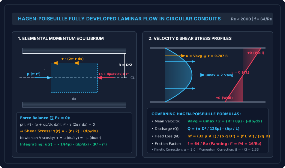
Figure 1: Hagen-Poiseuille Flow Structure & Profile Mechanics

The schematic below details the elemental fluid cylinder force equilibrium, linear shear stress distribution from zero at the pipe centerline to τ0\tau_0 at the wall, and the parabolic velocity profile with umax⁡=2Vavgu_{\max} = 2 V_{\text{avg}}.

Hagen-Poiseuille Flow Mechanics

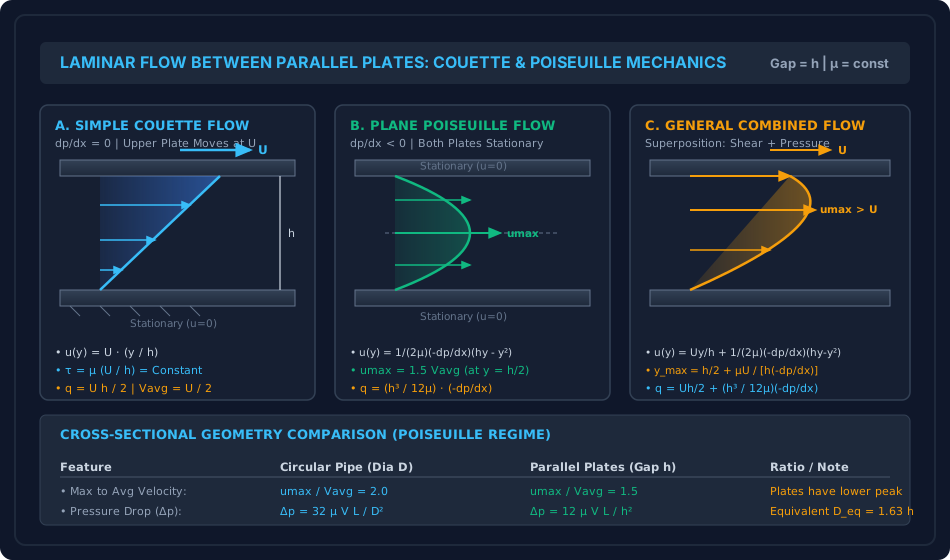
Figure 2: Parallel Plates Couette and Poiseuille Flow Regimes

The comparative diagram illustrates pure shear Couette flow, pure pressure-driven Poiseuille flow, and combined Couette-Poiseuille mechanics across the clearance gap hh.

Couette and Poiseuille Mechanics

6. Comparative Engineering Analysis & Parameter Regimes

The mathematical parameters governing laminar viscous flow across circular pipes and parallel plates are compared below:

Characteristic Parameter Circular Pipe (Diameter D=2RD = 2R) Parallel Plates (Gap Distance hh) Physical Significance & Exam Notes
Cross-Sectional Geometry Axi-symmetric circular tube (A=πR2A = \pi R^2) Planar slit of width B≫hB \gg h (A=BhA = B h) Boundary perimeter influences wall viscous retarding area.
Governing Equation 1rddr(rdudr)=1μdpdx\frac{1}{r}\frac{d}{dr}\left(r \frac{du}{dr}\right) = \frac{1}{\mu}\frac{dp}{dx} d2udy2=1μdpdx\frac{d^2 u}{dy^2} = \frac{1}{\mu}\frac{dp}{dx} Circular requires cylindrical coordinates.
Velocity Profile u(y)u(y) u(r)=umax⁡[1−(rR)2]u(r) = u_{\max}\left[1 - \left(\frac{r}{R}\right)^2\right] u(y)=12μ(−dpdx)(hy−y2)u(y) = \frac{1}{2\mu}\left(-\frac{dp}{dx}\right)(h y - y^2) Both profiles are quadratic parabolas.
Max to Mean Ratio (umax⁡/Vavgu_{\max} / V_{\text{avg}}) 2.002.00 1.501.50 (3/23/2) Crucial ratio for Pitot tube calibration.
Discharge Equation (QQ) Q=πD4128μ(−dpdx)Q = \frac{\pi D^4}{128 \mu}\left(-\frac{dp}{dx}\right) q=h312μ(−dpdx)q = \frac{h^3}{12\mu}\left(-\frac{dp}{dx}\right) Pipe scales as D4D^4; plates scale as h3h^3.
Pressure Drop (Δp\Delta p) Δp=32μVLD2\Delta p = \frac{32 \mu V L}{D^2} Δp=12μVLh2\Delta p = \frac{12 \mu V L}{h^2} Equivalent hydraulic diameter Deq=1.633hD_{\text{eq}} = 1.633 h.
Friction Factor (ff) f=64Ref = \frac{64}{Re} (where Re=ρVDμRe = \frac{\rho V D}{\mu}) f=96ReDhf = \frac{96}{Re_{D_h}} (where Dh=2h,Re=ρV(2h)μD_h = 2h, Re = \frac{\rho V (2h)}{\mu}) Derived from hf=fLDhV22gh_f = f \frac{L}{D_h}\frac{V^2}{2g}.
Kinetic Energy Factor (α\alpha) α=2.00\alpha = 2.00 α=1.543\alpha = 1.543 (54/3554/35) Energy flux correction due to velocity peak.
Momentum Factor (β\beta) β=1.333\beta = 1.333 (4/34/3) β=1.200\beta = 1.200 (6/56/5) Momentum flux correction factor.
Wall Shear Stress (τ0\tau_0) τ0=4μumax⁡R=8μVD\tau_0 = \frac{4 \mu u_{\max}}{R} = \frac{8 \mu V}{D} τ0=4μumax⁡h=6μVh\tau_0 = \frac{4 \mu u_{\max}}{h} = \frac{6 \mu V}{h} Direct shear stress exerted on containment boundaries.

7. Worked Numerical Examples (Pre-Calculated & Verified)

Problem 1: Industrial Oil Pipeline Sizing & Pumping Power (Hagen-Poiseuille)

Statement:
An industrial lubricating oil with dynamic viscosity μ=0.294 Pa⋅s\mu = 0.294\text{ Pa}\cdot\text{s} and specific gravity S=0.90S = 0.90 (ρ=900 kg/m3\rho = 900\text{ kg/m}^3) is pumped through a horizontal steel pipe of internal diameter D=100 mmD = 100\text{ mm} (0.10 m0.10\text{ m}) over a transmission length L=50 mL = 50\text{ m}. The volumetric flow rate is measured as Q=0.015708 m3/sQ = 0.015708\text{ m}^3\text{/s} (15.708 L/s15.708\text{ L/s}).

  1. Confirm whether the flow regime is strictly laminar.
  2. Determine the centerline maximum velocity umax⁡u_{\max} and locate the radial distance rr from the centerline where the local velocity equals the average velocity.
  3. Compute the wall shear stress τ0\tau_0, total pressure drop Δp\Delta p, head loss hfh_f, and required fluid pumping power PP.

Solution:

Step 1: Cross-Sectional Area and Mean Velocity

A=πD24=π(0.10)24=0.00785398 m2A = \frac{\pi D^2}{4} = \frac{\pi (0.10)^2}{4} = 0.00785398\text{ m}^2 Vavg=QA=0.015707963 m3/s0.00785398 m2=2.0000 m/sV_{\text{avg}} = \frac{Q}{A} = \frac{0.015707963\text{ m}^3\text{/s}}{0.00785398\text{ m}^2} = 2.0000\text{ m/s}

Step 2: Reynolds Number Verification

Re=ρVavgDμ=900 kg/m3×2.0000 m/s×0.10 m0.294 Pa⋅s=180.00.294=612.24Re = \frac{\rho V_{\text{avg}} D}{\mu} = \frac{900\text{ kg/m}^3 \times 2.0000\text{ m/s} \times 0.10\text{ m}}{0.294\text{ Pa}\cdot\text{s}} = \frac{180.0}{0.294} = 612.24

Since Re=612.24<2000Re = 612.24 < 2000, the flow is unambiguously in the laminar regime. Hagen-Poiseuille equations are strictly valid.

Step 3: Velocity Profile Parameters

  • Centerline maximum velocity: umax⁡=2×Vavg=2×2.0000 m/s=4.0000 m/su_{\max} = 2 \times V_{\text{avg}} = 2 \times 2.0000\text{ m/s} = 4.0000\text{ m/s}
  • Radial location where u(r)=Vavgu(r) = V_{\text{avg}}: u(r)=umax⁡[1−(rR)2]=umax⁡2  ⟹  rR=12≈0.7071u(r) = u_{\max} \left[1 - \left(\frac{r}{R}\right)^2\right] = \frac{u_{\max}}{2} \implies \frac{r}{R} = \frac{1}{\sqrt{2}} \approx 0.7071 R=D2=0.050 m=50.0 mmR = \frac{D}{2} = 0.050\text{ m} = 50.0\text{ mm} r=50.0 mm×0.707107=35.36 mmr = 50.0\text{ mm} \times 0.707107 = 35.36\text{ mm}

Step 4: Pressure Gradient, Total Pressure Drop, and Head Loss

dpdx=−32μVavgD2=−32×0.294×2.0000(0.10)2=−18.8160.01=−1881.60 Pa/m\frac{dp}{dx} = -\frac{32 \mu V_{\text{avg}}}{D^2} = -\frac{32 \times 0.294 \times 2.0000}{(0.10)^2} = -\frac{18.816}{0.01} = -1881.60\text{ Pa/m} Δp=(−dpdx)L=1881.60 Pa/m×50 m=94,080.00 Pa=94.08 kPa\Delta p = \left(-\frac{dp}{dx}\right) L = 1881.60\text{ Pa/m} \times 50\text{ m} = 94,080.00\text{ Pa} = 94.08\text{ kPa} hf=Δpρg=94080.00 N/m2900 kg/m3×9.81 m/s2=94080.008829.0=10.6558 m of oilh_f = \frac{\Delta p}{\rho g} = \frac{94080.00\text{ N/m}^2}{900\text{ kg/m}^3 \times 9.81\text{ m/s}^2} = \frac{94080.00}{8829.0} = 10.6558\text{ m of oil}

Step 5: Wall Shear Stress & Friction Factor

f=64Re=64612.24=0.104533f = \frac{64}{Re} = \frac{64}{612.24} = 0.104533 τ0=f8ρVavg2=0.1045338×900×(2.0)2=0.0130667×3600=47.04 Pa\tau_0 = \frac{f}{8} \rho V_{\text{avg}}^2 = \frac{0.104533}{8} \times 900 \times (2.0)^2 = 0.0130667 \times 3600 = 47.04\text{ Pa}

Alternative Verification:

τ0=−R2dpdx=0.0502×1881.60=0.025×1881.60=47.04 Pa(Exact Match)\tau_0 = -\frac{R}{2} \frac{dp}{dx} = \frac{0.050}{2} \times 1881.60 = 0.025 \times 1881.60 = 47.04\text{ Pa} \quad (\text{Exact Match})

Step 6: Pumping Power

P=Q×Δp=0.015707963 m3/s×94080.00 N/m2=1477.81 W=1.478 kWP = Q \times \Delta p = 0.015707963\text{ m}^3\text{/s} \times 94080.00\text{ N/m}^2 = 1477.81\text{ W} = 1.478\text{ kW}

Problem 2: Combined Couette-Poiseuille Flow Between Parallel Plates

Statement:
Two wide horizontal parallel plates are separated by a narrow clearance gap h=6.0 mmh = 6.0\text{ mm} (0.006 m0.006\text{ m}). The interspace is filled with heavy engine oil (μ=0.40 Pa⋅s\mu = 0.40\text{ Pa}\cdot\text{s}, ρ=880 kg/m3\rho = 880\text{ kg/m}^3). The bottom plate is fixed, while the upper plate translates steadily at U=1.80 m/sU = 1.80\text{ m/s}. Concurrently, a favorable longitudinal pressure gradient dpdx=−80,000 Pa/m\frac{dp}{dx} = -80,000\text{ Pa/m} (−80 kPa/m-80\text{ kPa/m}) acts along the channel.

  1. Determine the height ymax⁡y_{\max} above the bottom plate where the velocity reaches its maximum value, and compute umax⁡u_{\max}.
  2. Calculate the volumetric discharge per unit width (qq).
  3. Evaluate the shear stress at both the lower stationary plate and the upper moving plate.

Solution:

Step 1: Governing Velocity Distribution

u(y)=Uyh+12μ(−dpdx)(hy−y2)u(y) = U \frac{y}{h} + \frac{1}{2\mu}\left(-\frac{dp}{dx}\right)(h y - y^2) dudy=Uh+12μ(−dpdx)(h−2y)\frac{du}{dy} = \frac{U}{h} + \frac{1}{2\mu}\left(-\frac{dp}{dx}\right)(h - 2y)

Step 2: Position and Value of Maximum Velocity Setting dudy=0\frac{du}{dy} = 0:

0=1.800.006+800002×0.40(0.006−2y)0 = \frac{1.80}{0.006} + \frac{80000}{2 \times 0.40}(0.006 - 2y) 0=300+100000(0.006−2y)=300+600−200000y0 = 300 + 100000(0.006 - 2y) = 300 + 600 - 200000 y 200000y=900  ⟹  ymax⁡=900200000=0.00450 m=4.50 mm200000 y = 900 \implies y_{\max} = \frac{900}{200000} = 0.00450\text{ m} = 4.50\text{ mm}

Notice that 0<ymax⁡<6.0 mm0 < y_{\max} < 6.0\text{ mm}, confirming that maximum velocity occurs inside the clearance gap.

Substitute ymax⁡=0.0045 my_{\max} = 0.0045\text{ m} into u(y)u(y):

umax⁡=1.80(0.00450.006)+800000.80(0.006×0.0045−(0.0045)2)u_{\max} = 1.80 \left(\frac{0.0045}{0.006}\right) + \frac{80000}{0.80}\left(0.006 \times 0.0045 - (0.0045)^2\right) umax⁡=1.80×0.75+100000×(0.000027−0.00002025)=1.35+100000×(0.00000675)=1.35+0.675=2.0250 m/su_{\max} = 1.80 \times 0.75 + 100000 \times (0.000027 - 0.00002025) = 1.35 + 100000 \times (0.00000675) = 1.35 + 0.675 = 2.0250\text{ m/s}

(Note that umax⁡=2.025 m/s>U=1.80 m/su_{\max} = 2.025\text{ m/s} > U = 1.80\text{ m/s} due to the favorable pressure boost).

Step 3: Discharge per Unit Width (qq)

q=Uh2+h312μ(−dpdx)q = \frac{U h}{2} + \frac{h^3}{12\mu}\left(-\frac{dp}{dx}\right) q=1.80×0.0062+(0.006)3×8000012×0.40q = \frac{1.80 \times 0.006}{2} + \frac{(0.006)^3 \times 80000}{12 \times 0.40} q=0.005400+2.16×10−7×800004.80=0.005400+0.017284.80=0.005400+0.003600=0.009000 m3/(s⋅m)=9.00 L/(s⋅m)q = 0.005400 + \frac{2.16 \times 10^{-7} \times 80000}{4.80} = 0.005400 + \frac{0.01728}{4.80} = 0.005400 + 0.003600 = 0.009000\text{ m}^3\text{/(s}\cdot\text{m}) = 9.00\text{ L/(s}\cdot\text{m})

Step 4: Shear Stress Evaluation Using τ(y)=μdudy\tau(y) = \mu \frac{du}{dy}:

τ(y)=μ[Uh+12μ(−dpdx)(h−2y)]=μUh+(−dpdx)(h2−y)\tau(y) = \mu \left[\frac{U}{h} + \frac{1}{2\mu}\left(-\frac{dp}{dx}\right)(h - 2y)\right] = \frac{\mu U}{h} + \left(-\frac{dp}{dx}\right)\left(\frac{h}{2} - y\right)
  • At lower plate (y=0y = 0): τ(0)=0.40×1.800.006+80000×(0.0062−0)=120.0+80000×0.003=120.0+240.0=+360.00 Pa\tau(0) = \frac{0.40 \times 1.80}{0.006} + 80000 \times \left(\frac{0.006}{2} - 0\right) = 120.0 + 80000 \times 0.003 = 120.0 + 240.0 = +360.00\text{ Pa}
  • At upper plate (y=h=0.006 my = h = 0.006\text{ m}): τ(h)=0.40×1.800.006+80000×(0.003−0.006)=120.0−240.0=−120.00 Pa\tau(h) = \frac{0.40 \times 1.80}{0.006} + 80000 \times \left(0.003 - 0.006\right) = 120.0 - 240.0 = -120.00\text{ Pa}

(The negative sign indicates that shear stress on the fluid at the upper wall opposes the direction of plate translation, acting as viscous drag against the drive mechanism).


Problem 3: Concentric Sliding Sleeve & Viscous Dashpot Damping

Statement:
A vertical guide rod of outside diameter D=100.0 mmD = 100.0\text{ mm} (0.100 m0.100\text{ m}) supports a concentric cylindrical sliding sleeve of internal diameter dsleeve=101.6 mmd_{\text{sleeve}} = 101.6\text{ mm} (0.1016 m0.1016\text{ m}), length L=150 mmL = 150\text{ mm} (0.150 m0.150\text{ m}), and total mass M=2.50 kgM = 2.50\text{ kg}. The annular gap is filled with silicone damping oil of dynamic viscosity μ=0.150 Pa⋅s\mu = 0.150\text{ Pa}\cdot\text{s}.

  1. Calculate the uniform radial clearance cc.
  2. Derive the viscous damping coefficient CsleeveC_{\text{sleeve}} (in N⋅s/m\text{N}\cdot\text{s/m}) for the open sliding sleeve and determine its steady terminal fall velocity under gravity (g=9.81 m/s2g = 9.81\text{ m/s}^2).
  3. If the sleeve is instead fitted as a closed-end dashpot piston descending into a fixed cylinder of the same dimensions (forcing fluid upward through the narrow annular clearance), determine the hydraulic dashpot constant CdashpotC_{\text{dashpot}} and the new terminal velocity.

Solution:

Step 1: Radial Clearance

c=dsleeve−D2=0.1016−0.10002=0.00080 m=0.80 mmc = \frac{d_{\text{sleeve}} - D}{2} = \frac{0.1016 - 0.1000}{2} = 0.00080\text{ m} = 0.80\text{ mm}

Since c/D=0.0008/0.10=0.008≪1c/D = 0.0008 / 0.10 = 0.008 \ll 1, the annular slit can be unwrapped into a flat plane of width B=πD=π×0.10=0.314159 mB = \pi D = \pi \times 0.10 = 0.314159\text{ m}.

Step 2: Case A — Open Concentric Sliding Sleeve (Pure Shear Resistance) When falling at terminal velocity VtV_t, gravity force equals the viscous wall shear force:

W=Mg=2.50 kg×9.81 m/s2=24.525 NW = M g = 2.50\text{ kg} \times 9.81\text{ m/s}^2 = 24.525\text{ N}

The shear stress across the thin clearance cc is purely Couette:

τ=μVtc\tau = \mu \frac{V_t}{c}

The shear area is As=πDLA_s = \pi D L:

Fshear=τAs=(μVtc)(πDL)=(μπDLc)VtF_{\text{shear}} = \tau A_s = \left(\mu \frac{V_t}{c}\right) (\pi D L) = \left(\frac{\mu \pi D L}{c}\right) V_t

The damping coefficient is:

Csleeve=μπDLc=0.150×π×0.10×0.1500.00080=0.007068580.00080=8.8357 N⋅s/mC_{\text{sleeve}} = \frac{\mu \pi D L}{c} = \frac{0.150 \times \pi \times 0.10 \times 0.150}{0.00080} = \frac{0.00706858}{0.00080} = 8.8357\text{ N}\cdot\text{s/m}

Terminal velocity:

Vt=WCsleeve=24.525 N8.8357 N⋅s/m=2.7757 m/sV_t = \frac{W}{C_{\text{sleeve}}} = \frac{24.525\text{ N}}{8.8357\text{ N}\cdot\text{s/m}} = 2.7757\text{ m/s}

Step 3: Case B — Closed-End Dashpot Piston (Displacement-Driven Annular Backflow) When the bottom is closed, the descending piston displaces fluid volume at rate:

Qdisp=ApVt=(πD24)VtQ_{\text{disp}} = A_p V_t = \left(\frac{\pi D^2}{4}\right) V_t

This displaced volume must escape upward through the narrow annular slit of width B=πDB = \pi D and gap cc. From parallel-plate Poiseuille discharge (q=c312μΔpLq = \frac{c^3}{12\mu}\frac{\Delta p}{L}):

Qup=Bq=(πD)c312μΔpLQ_{\text{up}} = B q = (\pi D) \frac{c^3}{12\mu}\frac{\Delta p}{L}

Equating Qup=QdispQ_{\text{up}} = Q_{\text{disp}}:

(πD24)Vt=πDc312μLΔp  ⟹  Δp=3μLDc3Vt\left(\frac{\pi D^2}{4}\right) V_t = \frac{\pi D c^3}{12\mu L} \Delta p \implies \Delta p = \frac{3 \mu L D}{c^3} V_t

The resulting upward pressure force acting on the piston base is:

Fpressure=Δp⋅Ap=(3μLDc3Vt)(πD24)=(3πμLD34c3)VtF_{\text{pressure}} = \Delta p \cdot A_p = \left(\frac{3 \mu L D}{c^3} V_t\right) \left(\frac{\pi D^2}{4}\right) = \left(\frac{3 \pi \mu L D^3}{4 c^3}\right) V_t

Evaluating the pressure damping stiffness kpk_p:

kp=3π×0.150×0.150×(0.10)34×(0.00080)3=0.00021205754×5.12×10−10=0.00021205752.048×10−9=103,543.71 N⋅s/mk_p = \frac{3 \pi \times 0.150 \times 0.150 \times (0.10)^3}{4 \times (0.00080)^3} = \frac{0.0002120575}{4 \times 5.12 \times 10^{-10}} = \frac{0.0002120575}{2.048 \times 10^{-9}} = 103,543.71\text{ N}\cdot\text{s/m}

Total damping constant:

Cdashpot≈kp+ks=103,543.71+1,665.53=105,209.24 N⋅s/mC_{\text{dashpot}} \approx k_p + k_s = 103,543.71 + 1,665.53 = 105,209.24\text{ N}\cdot\text{s/m}

The resulting terminal velocity in the closed dashpot:

Vt,dashpot=WCdashpot=24.525 N105,209.24 N⋅s/m=0.0002331 m/s=0.233 mm/sV_{t,\text{dashpot}} = \frac{W}{C_{\text{dashpot}}} = \frac{24.525\text{ N}}{105,209.24\text{ N}\cdot\text{s/m}} = 0.0002331\text{ m/s} = 0.233\text{ mm/s}

Physical Engineering Insight: Constraining the displaced fluid through the annular gap increases damping resistance by a factor of 1052098.84≈11,900\frac{105209}{8.84} \approx 11,900, reducing velocity from 2.78 m/s2.78\text{ m/s} to a controlled crawl of 0.233 mm/s0.233\text{ mm/s}. This demonstrates the fundamental principle of seismic viscous dampers in civil structures.


8. High-Yield Examination Traps & Ambiguities

S.No. Trap / Common Misconception Correct Technical Reality Examination Occurrence
1 Darcy ff vs Fanning f′f' Friction Factor: Confusing ff with f′f'. Darcy friction factor is f=64Ref = \frac{64}{Re} (hf=fLV22gDh_f = \frac{f L V^2}{2g D}). Fanning friction factor is f′=cf=f4=16Ref' = c_f = \frac{f}{4} = \frac{16}{Re} (τ0=12cfρV2\tau_0 = \frac{1}{2} c_f \rho V^2). GATE/ESE explicitly test this fourfold difference! GATE CE, ESE Prelims
2 Shear Stress Variation Across Pipe: Assuming shear stress is parabolic like velocity. Shear stress is strictly linear across the radius: τ(r)=−r2dpdx\tau(r) = -\frac{r}{2}\frac{dp}{dx}. It is ZERO at the pipe centerline and MAXIMUM at the pipe wall. SSC JE, State AE
3 Energy Correction Factor α\alpha: Assuming α=1.0\alpha = 1.0 for all pipe flows. For laminar circular pipe flow, α=2.00\alpha = 2.00 and β=1.333\beta = 1.333. Neglecting α\alpha introduces a 100%100\% error in kinetic energy head (αV22g=2V22g=V2g\frac{\alpha V^2}{2g} = \frac{2 V^2}{2g} = \frac{V^2}{g}). In turbulent flow, α≈1.058\alpha \approx 1.058. GATE CE, UPSC ESE
4 Velocity Ratio in Pipes vs Plates: Applying umax⁡/Vavg=2.0u_{\max}/V_{\text{avg}} = 2.0 to parallel plates. In circular pipes, umax⁡=2.0Vavgu_{\max} = 2.0 V_{\text{avg}}. In parallel plates, umax⁡=1.50Vavgu_{\max} = 1.50 V_{\text{avg}} (3/23/2). In open channels, umax⁡≈1.15Vavgu_{\max} \approx 1.15 V_{\text{avg}}. SSC JE, RRB JE, ESE
5 Inclined Pipes & Gravity: Inserting purely static pressure pp instead of piezometric pressure p∗p^*. In inclined pipes, flow is driven by the piezometric gradient: d(p+γz)dx\frac{d(p + \gamma z)}{dx}. The Hagen-Poiseuille formula becomes: hf=32μVLγD2=(z1−z2)+p1−p2γh_f = \frac{32 \mu V L}{\gamma D^2} = (z_1 - z_2) + \frac{p_1 - p_2}{\gamma}. GATE CE, ESE Mains
6 Pitot Tube Location for Mean Velocity: Placing Pitot tube at r=0.5Rr = 0.5 R. u(r)=Vavgu(r) = V_{\text{avg}} occurs at r=R2≈0.7071Rr = \frac{R}{\sqrt{2}} \approx 0.7071 R (not at the mid-radius 0.5R0.5 R, where u(0.5R)=0.75umax⁡=1.5Vavgu(0.5R) = 0.75 u_{\max} = 1.5 V_{\text{avg}}!). GATE CE

9. Real-World Engineering Applications & Case Studies

  1. Fluid Film Lubrication & Journal Bearings:
    Hydrodynamic journal bearings in high-head hydroelectric turbines (Francis and Pelton runner shafts) rely on Couette-Poiseuille flow in the eccentric clearance between the rotating shaft and the stationary bearing bush. The converging clearance generates hydrodynamic pressures exceeding 15–30 MPa15\text{--}30\text{ MPa}, preventing metal-to-metal contact.
  2. Long-Distance Heavy Crude Oil Pipelines:
    High-viscosity crude oils (μ>0.1–1.0 Pa⋅s\mu > 0.1\text{--}1.0\text{ Pa}\cdot\text{s}) transported through pipelines operate strictly in the Hagen-Poiseuille laminar regime. Because head loss scales inversely with diameter to the fourth power (hf∝1/D4h_f \propto 1/D^4), a modest 15%15\% increase in pipeline diameter reduces pumping pressure and power requirements by over 46%46\%.
  3. Seismic Viscous Dampers for Bridges & Tall Buildings:
    Fluid viscous dampers (FVDs) installed at bridge expansion joints and structural bracing frames utilize concentric dashpot pistons forcing silicone fluids through annular orifices. As demonstrated in Problem 3, the resulting damping force Fd=CVαF_d = C V^\alpha dissipates earthquake energy through laminar viscous shear without adding structural stiffness.
  4. Microfluidics, Environmental Filters & Soil Permeability:
    Laminar viscous flow through narrow conduits forms the physical basis of Darcy's Law for groundwater seepage through soil pore channels (effective diameter d10d_{10}), slow sand water filtration, and microfluidic lab-on-a-chip environmental sensors.

10. Cross-Disciplinary & Downstream Dependencies

[Fluid Mechanics: Ch 06 Laminar Flow]
        │
        ├──► [Subject 08: Geotechnical Engineering]
        │         └─► Soil Permeability & Seepage (Darcy's Law derived from Hagen-Poiseuille in soil pores)
        │
        ├──► [Subject 09: Environmental Engineering]
        │         ├─► Type-I Discrete Particle Settling (Stokes' Law: CD = 24/Re)
        │         └─► Slow Sand Filtration & Pipe Network Head Losses
        │
        ├──► [Subject 03: Structural Analysis]
        │         └─► Seismic Isolation & Viscous Fluid Dampers (Energy Dissipation)
        │
        └──► [Fluid Mechanics: Ch 07 Boundary Layer Theory]
                  └─► Laminar Boundary Layer on Flat Plates (Blasius Equation)

11. Summary Formula Cheat Sheet & Memory Anchors

  • Hagen-Poiseuille Circular Pipe:

    • Shear Stress: τ(r)=−r2dpdx  ⟹  τ0=−R2dpdx=4μumax⁡R\tau(r) = -\frac{r}{2}\frac{dp}{dx} \implies \tau_0 = -\frac{R}{2}\frac{dp}{dx} = \frac{4\mu u_{\max}}{R}
    • Velocity Profile: u(r)=umax⁡[1−(rR)2]u(r) = u_{\max}\left[1 - \left(\frac{r}{R}\right)^2\right]
    • Ratio: umax⁡=2.0Vavgu_{\max} = 2.0 V_{\text{avg}}
    • Mean Velocity Position: r=R2≈0.7071Rr = \frac{R}{\sqrt{2}} \approx 0.7071 R
    • Discharge: Q=πD4128μ(−dpdx)Q = \frac{\pi D^4}{128 \mu}\left(-\frac{dp}{dx}\right)
    • Head Loss: hf=32μVLγD2=fLV22gDh_f = \frac{32 \mu V L}{\gamma D^2} = \frac{f L V^2}{2g D}
    • Darcy Friction Factor: f=64Ref = \frac{64}{Re} | Fanning: f′=16Ref' = \frac{16}{Re}
    • Energy & Momentum Factors: α=2.00,β=43≈1.333\alpha = 2.00, \quad \beta = \frac{4}{3} \approx 1.333
  • Plane Poiseuille (Parallel Plates Gap hh):

    • Velocity Profile: u(y)=12μ(−dpdx)(hy−y2)u(y) = \frac{1}{2\mu}\left(-\frac{dp}{dx}\right)(h y - y^2)
    • Ratio: umax⁡=1.50Vavgu_{\max} = 1.50 V_{\text{avg}}
    • Discharge per unit width: q=h312μ(−dpdx)q = \frac{h^3}{12\mu}\left(-\frac{dp}{dx}\right)
    • Head Loss: hf=12μVLγh2h_f = \frac{12 \mu V L}{\gamma h^2}
    • Factors: α=5435≈1.543,β=65=1.200\alpha = \frac{54}{35} \approx 1.543, \quad \beta = \frac{6}{5} = 1.200
  • Combined Couette-Poiseuille:

    • Velocity: u(y)=Uyh+12μ(−dpdx)(hy−y2)u(y) = U \frac{y}{h} + \frac{1}{2\mu}\left(-\frac{dp}{dx}\right)(h y - y^2)
    • Backflow Threshold: dpdx≥2μUh2\frac{dp}{dx} \ge \frac{2\mu U}{h^2}

12. Comprehensive References & Standard Codes

  1. White, F. M. (2016). Fluid Mechanics, 8th Edition, McGraw-Hill Education. (Chapter 6: Viscous Flow in Ducts).
  2. Streeter, V. L., Wylie, E. B., & Bedford, K. W. (1998). Fluid Mechanics, 9th Edition, McGraw-Hill.
  3. Modi, P. N., & Seth, S. M. (2018). Hydraulics and Fluid Mechanics Including Hydraulics Machines, Standard Book House, New Delhi. (Chapter 11: Laminar Flow).
  4. Fox, R. W., McDonald, A. T., & Pritchard, P. J. (2015). Introduction to Fluid Mechanics, 9th Edition, John Wiley & Sons.
  5. IS 456:2000 & IS 13920:2016 (Bureau of Indian Standards: Structural Damping & Dynamic Isolation Standards).