Turbulent Pipe Flow, Darcy-Weisbach Equation, Moody Diagram & Pipe Roughness
In this chapter (4 topics)
On this page
- 1. Module Overview & Pedagogical Scope
- 2. Official Examination Syllabus Mapping
- 3. Fundamental Physical Principles & Governing Assumptions
- 4. Mathematical Derivations & Rigorous Proofs
- Sub-derivation A: Reynolds Decomposition, Reynolds Stresses & Prandtl Mixing Length
- Sub-derivation B: The Universal Law of the Wall
- Sub-derivation C: Velocity Defect Law & Mean Velocity
- Sub-derivation D: Hydrodynamic Roughness Regimes (Nikuradse Criteria)
- Sub-derivation E: Friction Factor Formulations & The Moody Chart
- 5. Technical Diagrams & Interactive Architectural Schematics
- Figure 1: Near-Wall Sublayer Structure & Nikuradse Roughness Regimes
- Figure 2: The Moody Diagram Architecture
- 6. Comparative Engineering Analysis & Parameter Regimes
- 7. Worked Numerical Examples (Pre-Calculated & Verified)
- Problem 1: Boundary Classification & Viscous Sublayer Thickness
- Problem 2: Logarithmic Velocity Profile & Velocity Defect
- Problem 3: Commercial Penstock Sizing (Colebrook-White vs Swamee-Jain)
- 8. High-Yield Examination Traps & Ambiguities
- 9. Real-World Engineering Applications & Case Studies
- 10. Cross-Disciplinary & Downstream Dependencies
- 11. Summary Formula Cheat Sheet & Memory Anchors
- 12. Comprehensive References & Standard Codes
1. Module Overview & Pedagogical Scope
Turbulent flow represents the predominant fluid dynamic regime in municipal water supply networks, hydroelectric penstocks, industrial transport conduits, and environmental pipelines. When the conduit Reynolds number exceeds the critical threshold (), infinitesimal disturbances undergo exponential amplification, destroying laminar laminae and establishing a chaotic, three-dimensional, rotational flow field characterized by intense continuous velocity fluctuations:
In turbulent pipe flow, momentum transfer is dominated by macroscopic eddy mixing rather than molecular diffusion. This produces a much flatter, fuller velocity profile across the conduit core and exceptionally steep velocity gradients confined to a microscopic near-wall boundary layer.
This module delivers a comprehensive mathematical and engineering treatment of:
- Turbulence Physics & Reynolds Stresses: Reynolds averaging, the apparent turbulent shear stress tensor (), and Prandtl's mixing length hypothesis.
- Universal Law of the Wall: Asymptotic three-zone boundary layer structure (viscous sublayer, buffer zone, and logarithmic overlap layer), and Prandtl's velocity defect law.
- Hydrodynamic Roughness Regimes (Nikuradse Criteria): The physical interplay between equivalent sand roughness height and viscous sublayer thickness , establishing the exact boundaries between hydrodynamically smooth, transitional, and completely rough regimes.
- Friction Factor Formulations & The Moody Diagram: Exact analytical equations (Blasius, von Kármán-Prandtl smooth, Nikuradse rough), the implicit Colebrook-White equation, and explicit engineering approximations (Swamee-Jain, Haaland) for municipal conduit design.
2. Official Examination Syllabus Mapping
Website note: this mapping is from the author’s notes. It has not been checked against the official notification for each examination; confirm the current syllabus with the examining body.
| Examination Body | Syllabus Clause / Core Topic Reference | Focus Regimes & Weightage |
|---|---|---|
| GATE CE (IITs / IISc) | Fluid Mechanics: Turbulent flow in pipes; Darcy-Weisbach equation; Moody chart; boundary layer thickness; velocity profiles in smooth and rough pipes; friction factor. | Critical Core Subject (1 to 2 questions annually; friction factor calculations, smooth vs rough classifications, Colebrook iteration). |
| UPSC ESE (Prelims & Mains) | Paper-II Fluid Mechanics: Turbulent flow through pipes; Reynolds stress; Prandtl mixing length; velocity defect; hydrodynamically smooth and rough boundaries; age effect on pipes. | Extremely High (20–25 marks in Mains subjective; 3–5 MCQs in Prelims). |
| SSC JE & State AE / JE | Concept of turbulent flow, Darcy-Weisbach formula, Chezy formula, loss of head due to friction, hydraulic gradient line, Moody chart. | High Frequency (Direct formula questions: , smooth vs rough values). |
| RRB JE (CBT-2) | Pipe flow, head loss, friction factor variation with Reynolds number and roughness. | Standard MCQs on friction factor trends. |
3. Fundamental Physical Principles & Governing Assumptions
- High Reynolds Number Flow: The flow occurs well above the critical transition regime ().
- Reynolds Time-Averaging (RANS Formulation): Instantaneous flow variables are decomposed into steady time-mean components () and turbulent fluctuating components (), where by definition:
- Fully Developed Core Flow: The pipe is of uniform diameter and sufficient length () such that entrance effects have decayed and the time-averaged velocity profile is invariant with axial distance .
- Isotropic Homogeneous Fluid: The fluid is continuous, homogeneous, and Newtonian ().
- No-Slip Boundary Condition at Wall: At the solid conduit boundary (), both mean and fluctuating velocities vanish identically: .
4. Mathematical Derivations & Rigorous Proofs
Sub-derivation A: Reynolds Decomposition, Reynolds Stresses & Prandtl Mixing Length
Consider the instantaneous Navier-Stokes momentum equation along the longitudinal flow coordinate . Decomposing velocities into mean and fluctuating parts (, ) and time-averaging over a characteristic turbulent timescale :
The bracketed term represents the total effective shear stress:
The extra convective momentum transfer term:
is known as the Reynolds Apparent Turbulent Shear Stress.
Physical Origin of :
When a fluid lump moves upward from a lower layer (), it arrives at a faster layer with a velocity deficit (). Thus, the product . Conversely, when a lump moves downward (), it brings excess momentum (), again yielding . Therefore, the time-averaged correlation is negative, rendering strictly positive.
Prandtl's Mixing Length Hypothesis:
In 1925, Ludwig Prandtl postulated that a turbulent fluid lump retains its original momentum over a characteristic transverse distance (the mixing length) before coalescing with surrounding fluid:
Substituting this into the Reynolds stress expression:
Near a solid boundary, Prandtl reasoned on dimensional grounds that the eddy scale is constrained by the distance to the wall:
where is the dimensionless von Kármán constant.
Sub-derivation B: The Universal Law of the Wall
Near the pipe wall (), the shear stress is approximately constant and equal to the wall shear stress: .
Define the characteristic scaling parameters:
- Shear Velocity (Friction Velocity):
- Dimensionless Distance from Wall:
- Dimensionless Velocity:
The turbulent boundary layer resolves into three distinct asymptotic sublayers:
1. Viscous Sublayer ():
Adjacent to the wall, turbulent fluctuations are damped out by wall proximity. Viscous shear stress completely dominates (). Integrating:
The velocity varies linearly with distance from the wall.
2. Buffer Layer ():
In this transition zone, molecular viscous stress and Reynolds turbulent stress are of the same order of magnitude. No simple analytical equation exists.
3. Logarithmic Overlap Layer ():
Turbulent Reynolds shear dominates completely ( with ):
Integrating with respect to :
Dividing by :
Substituting experimental constants and (Nikuradse, 1933):
This is the celebrated Prandtl-von Kármán Universal Law of the Wall.
Sub-derivation C: Velocity Defect Law & Mean Velocity
At the pipe centerline (), the velocity reaches its maximum value :
Subtracting the local velocity equation from the centerline equation eliminates the wall roughness constant :
This is von Kármán's Velocity Defect Law. Remarkably, this defect profile is universal—it holds identically for both hydrodynamically smooth and completely rough conduits!
Average Flow Velocity ():
Integrating the defect profile over the pipe cross-section ():
Radial Position of Mean Velocity:
Equating local velocity to mean velocity:
Radial distance from centerline:
Key Comparison for Civil Engineering Exams:
- In Laminar Flow (Hagen-Poiseuille): occurs at .
- In Turbulent Flow (Logarithmic): occurs at .
Sub-derivation D: Hydrodynamic Roughness Regimes (Nikuradse Criteria)
The thickness of the laminar/viscous sublayer is formally defined as the distance where the linear sublayer matches the logarithmic profile ():
J. Nikuradse (1933) systematically coated pipe interiors with graded uniform sand grains of diameter and established three hydrodynamic roughness regimes based on the ratio of sand roughness height to sublayer thickness:
| Hydrodynamic Regime | Relative Sublayer Criteria | Roughness Reynolds Number | Physical Flow Mechanism & Governing Friction Factor |
|---|---|---|---|
| Hydrodynamically Smooth Boundary | Sand grains are completely submerged inside the quiescent viscous sublayer. Boundary behaves as if hydraulically polished. Friction factor depends only on Reynolds number: . | ||
| Transition Regime | Roughness peaks emerge partially into the buffer layer. Form drag on asperities and viscous wall shear coexist. Friction factor depends on both Reynolds number and relative roughness: . | ||
| Completely Rough Boundary | Roughness peaks completely project beyond the sublayer, destroying it. Flow resistance is governed entirely by pressure form drag (wake shedding behind asperities). Friction factor is independent of Reynolds number: only. |
Sub-derivation E: Friction Factor Formulations & The Moody Chart
The Darcy-Weisbach head loss equation is defined as:
where is the dimensionless Darcy friction factor. (Note: Fanning friction factor , wall shear stress ).
1. Blasius Formula (Smooth Pipes, ):
Empirical formula derived by Heinrich Blasius (1913):
2. Kármán-Prandtl Resistance Equation for Smooth Pipes:
Derived from the logarithmic law of the wall:
3. Nikuradse Resistance Equation for Completely Rough Pipes:
When the viscous sublayer is completely destroyed (), viscosity drops out of the problem:
4. Colebrook-White Transition Formula (1939):
C. F. Colebrook and C. M. White devised an ingenious transcendental equation that smoothly bridges the Kármán-Prandtl smooth equation and the Nikuradse rough equation across the entire commercial transition regime:
This equation is the mathematical foundation of Lewis F. Moody's celebrated Moody Diagram (1944).
5. Explicit Engineering Approximations:
Because the Colebrook-White equation is implicit in , engineers utilize accurate explicit approximations:
- Swamee-Jain Equation (1976) (Accurate within for and ):
- Haaland Equation (1983):
5. Technical Diagrams & Interactive Architectural Schematics
Figure 1: Near-Wall Sublayer Structure & Nikuradse Roughness Regimes
The diagram below illustrates the three-zone boundary layer structure (, buffer, and core), and the physical mechanism distinguishing hydrodynamically smooth, transition, and completely rough boundaries.
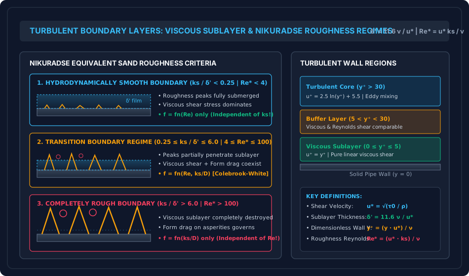
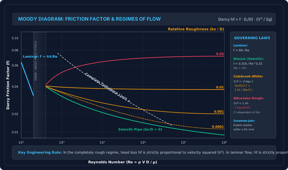
Figure 2: The Moody Diagram Architecture
The comprehensive Moody chart below displays the log-log mapping of Darcy friction factor across Reynolds numbers from to , depicting laminar flow (), the critical transition zone, smooth conduit limits, and the complete turbulence asymptote.
6. Comparative Engineering Analysis & Parameter Regimes
| Flow Property / Feature | Laminar Pipe Flow () | Turbulent Pipe Flow () |
|---|---|---|
| Momentum Transport Mechanism | Molecular diffusion () | Macroscopic eddy mixing () |
| Velocity Profile Geometry | Quadratic Parabola: | Logarithmic / 1/7th Power Law: |
| Centerline-to-Mean Ratio () | Exactly | (Typically ) |
| Mean Velocity Radial Location () | ||
| Kinetic Energy Factor () | (Taken as ) | |
| Momentum Correction Factor () | () | () |
| Friction Factor Dependence | (Strictly independent of roughness ) | (Becomes independent of in rough regime) |
| Head Loss Dependence on Velocity | (Linear with velocity) | (Smooth) to (Completely rough) |
| Shear Stress Variation Across Pipe | Linear from 0 at CL to at wall | Linear from 0 at CL to at wall (Fundamental momentum identity!) |
7. Worked Numerical Examples (Pre-Calculated & Verified)
Problem 1: Boundary Classification & Viscous Sublayer Thickness
Statement:
Clean water at () flows through a horizontal municipal pipe of diameter () at an average flow velocity . The measured Darcy friction factor is .
- Compute the wall shear stress and the friction velocity (shear velocity) .
- Calculate the nominal thickness of the viscous sublayer .
- Determine the hydrodynamic boundary classification if the pipeline is constructed of:
- Case (a): Drawn smooth brass tubing ().
- Case (b): Commercial galvanized iron pipe ().
- Case (c): Severely tuberculated cast iron main ().
Solution:
Step 1: Wall Shear Stress and Shear Velocity
(Check: . Exact match).
Step 2: Viscous Sublayer Thickness
Step 3: Hydrodynamic Classification for Each Roughness Case
-
Case (a): Drawn Smooth Tubing ():
Since and , the pipe behaves as HYDRODYNAMICALLY SMOOTH. The roughness peaks are fully submerged within the viscous sublayer.
-
Case (b): Galvanized Iron ():
Since and , the pipe operates in the TRANSITION REGIME. Friction depends simultaneously on and .
-
Case (c): Tuberculated Cast Iron ():
Since and , the pipe is COMPLETELY ROUGH. The viscous sublayer is totally annihilated by eddy shedding; is independent of .
Problem 2: Logarithmic Velocity Profile & Velocity Defect
Statement:
In a turbulent pipe flow of air through a smooth duct of internal radius (), the measured centerline maximum velocity is and the shear velocity is .
Using von Kármán's universal velocity defect law:
- Compute the local time-averaged flow velocity at distance and from the duct boundary.
- Calculate the cross-sectional mean velocity and the ratio .
- Determine the radial coordinate where local velocity equals the mean flow velocity.
Solution:
Step 1: Local Velocities Across Conduit
-
At (radial position ):
-
At (mid-radius position ):
Step 2: Cross-Sectional Mean Flow Velocity
(Compare with laminar flow where ; the turbulent profile is significantly more uniform).
Step 3: Radial Position of Mean Velocity
Radial distance from centerline:
Problem 3: Commercial Penstock Sizing (Colebrook-White vs Swamee-Jain)
Statement:
A hydroelectric penstock constructed of commercial welded steel has diameter () and length . It conveys water () at design discharge . The absolute roughness of the steel conduit is ().
- Determine the relative pipe roughness and the flow Reynolds number .
- Calculate the Darcy friction factor using the explicit Swamee-Jain formula, and verify convergence using the implicit Colebrook-White equation.
- Compute the friction head loss , hydraulic gradient slope , and the pumping power lost to viscous friction.
Solution:
Step 1: Flow Kinematics and Reynolds Number
Since , flow is highly turbulent. Relative roughness:
Step 2: Explicit Swamee-Jain Friction Factor Calculation
Step 3: Colebrook-White Implicit Convergence
Using :
Second iteration yields exact convergence to 5 figures:
The Swamee-Jain formula provides an outstanding agreement within error!
Step 4: Friction Head Loss, Hydraulic Slope & Dissipated Power
Pumping power lost to friction:
8. High-Yield Examination Traps & Ambiguities
| S.No. | Examination Trap / Confusion | Rigorous Engineering Distinction | Primary Exam |
|---|---|---|---|
| 1 | Smooth vs Rough Pipe Definition: Believing that a pipe made of "rough" material is always rough. | A pipe is hydrodynamically smooth if , regardless of the material! At low velocities, is large, submerging the roughness. At high velocities, increases, shrinks, and the exact same pipe becomes hydrodynamically rough! | GATE CE, UPSC ESE |
| 2 | Friction Factor Independence on : Stating always decreases with . | In the completely rough regime, the Moody curves are completely horizontal; is strictly independent of and depends solely on . | SSC JE, State AE |
| 3 | Linear vs Parabolic Shear Stress: Assuming turbulent shear stress varies non-linearly across the pipe. | The total shear stress is strictly linear across the conduit in both laminar AND turbulent flows (dictated purely by static equilibrium ). Only the split between laminar and turbulent components changes. | GATE CE, ESE Mains |
| 4 | Velocity Ratio (): Using for turbulent flow. | In laminar flow, . In turbulent pipe flow, . | SSC JE, RRB JE |
| 5 | Fanning vs Darcy Friction Factor: Writing . | In British/American literature, . Ensure whether the exam question provides Darcy friction factor () or coefficient of friction (). | GATE CE, ESE Prelims |
9. Real-World Engineering Applications & Case Studies
- Water Distribution Networks & Conduit Aging (Tuberculation):
Over 20–50 years of municipal service, unlined cast iron water mains suffer internal corrosion and bio-chemical encrustation (tuberculation). Absolute roughness increases from (new) to (aged), causing friction factor to double and carrying capacity to drop by over . - Hydraulic Penstocks in Hydroelectric Stations:
In high-head hydroelectric plants, water velocities exceed . Under these high shear velocities (), the sublayer shrinks below , forcing the penstock into the completely rough regime. Smooth epoxy or polyurethane internal linings are applied to suppress roughness and conserve millions of kilowatt-hours annually. - Slurry Pipelines & Dredging Conduits:
Mining slurry pipelines transporting fly ash, copper tailings, or dredged silt require turbulent suspension velocities to prevent sedimentation. Operating at , friction factor calculations directly dictate booster pump station spacing along hundreds of kilometers.
10. Cross-Disciplinary & Downstream Dependencies
[Fluid Mechanics: Ch 06 Turbulent Pipe Flow]
        │
        ├──► [Subject 09: Environmental Engineering]
        │         ├─► Water Supply Networks (Hardy Cross Analysis, Hazen-Williams vs Darcy)
        │         └─► Sewer Line Self-Cleansing Velocities & Friction Slopes
        │
        ├──► [Subject 04: Water Resources & Hydrology]
        │         └─► Penstock Hydraulics, Surge Tank Dynamics & Hydraulic Turbines
        │
        ├──► [Fluid Mechanics: Ch 06 Topic 03]
        │         └─► Minor Losses, Parallel Pipes & Equivalent Pipe Formulations
        │
        └──► [Fluid Mechanics: Ch 07 Boundary Layer Theory]
                  └─► Turbulent Boundary Layer on Flat Plates & Form Drag
11. Summary Formula Cheat Sheet & Memory Anchors
- Reynolds Stress & Mixing Length:
- Friction Velocity & Sublayer:
- Nikuradse Roughness Boundaries:
- Smooth:
- Transition:
- Rough:
- Universal Velocity Defect:
- Friction Factors:
- Blasius (Smooth, ):
- Nikuradse (Rough):
- Colebrook-White:
- Swamee-Jain Explicit:
12. Comprehensive References & Standard Codes
- Moody, L. F. (1944). Friction Factors for Pipe Flow, Transactions of the ASME, Vol. 66, pp. 671–684.
- Colebrook, C. F. (1939). Turbulent Flow in Pipes, with Particular Reference to the Transition Region Between the Smooth and Rough Pipe Laws, Journal of the ICE, Vol. 11, pp. 133–156.
- Nikuradse, J. (1933). Laws of Flow in Rough Pipes, VDI-Forschungsheft 361. (NACA TM 1292).
- White, F. M. (2016). Fluid Mechanics, 8th Edition, McGraw-Hill Education.
- IS 7784 & IS 4880 (Bureau of Indian Standards: Codes of Practice for Design of Tunnels, Shafts and Water Conduits).