Kinematics of Fluid Deformation — Rotation, Vorticity, Circulation & Strain Rates
In this chapter (5 topics)
On this page
- 1. Topic Metadata Table
- 2. Executive Summary
- 3. General Helmholtz Decomposition of Fluid Motion
- 4. Rate of Strain Tensor & Deformation Components
- 4.1 Linear Strain Rates (Extensional Deformation)
- 4.2 Volumetric Dilatation Rate
- 4.3 Angular Strain Rate (Shear Deformation)
- 5. Rotation Vector & Vorticity Tensor
- 5.1 Fluid Rotation Vector (vecω)
- 5.2 Vorticity Vector (vecζ)
- 5.3 Physical Criterion: Rotational vs. Irrotational Flow
- 6. Circulation & Stokes' Theorem
- 6.1 Definition of Circulation (Γ)
- 6.2 Stokes' Theorem Bridge
- 7. Kinematic Analysis of Vortices: Forced Vortex vs Free (Potential) Vortex
- Detailed Kinematic Comparison Matrix
- 8. Visual Diagrams & Architectural Schematics
- 8.1 Helmholtz Decomposition of Fluid Element Motion
- 8.2 Vorticity, Circulation, Stokes' Theorem & Vortex Regimes
- 9. Step-by-Step Numerical Problems with Complete Calculations
- Problem 1: 2D Deformation Tensor & Irrotationality Check
- Problem 2: Laminar Couette Shear Flow & Stokes' Theorem Verification
- Problem 3: Forced Vortex vs Free Vortex Vorticity & Circulation
- 10. High-Yield Exam Pitfalls, Traps & Shortcuts
- 11. Multi-Exam Question Bank (GATE, ESE, SSC JE, State AE, RRB JE)
- Question 1 (GATE CE — Analytical)
- Question 2 (UPSC ESE Paper-II — Descriptive / Analytical)
- Question 3 (SSC JE — Direct Conceptual)
- Question 4 (State PSC AE — Numerical)
- Question 5 (RRB JE — Direct Knowledge)
- 12. Comprehensive Summary, Formula Cheatsheet & Academic References
- 12.1 Formula Cheatsheet
- 12.2 Academic & Standard References
1. Topic Metadata Table
| Field | Detail |
|---|---|
| Subject | Fluid Mechanics & Hydraulic Machinery (Subject 07) |
| Chapter | Chapter 03: Fluid Kinematics |
| Topic Code | FM-03-04 |
| Topic Title | Kinematics of Fluid Deformation: Linear Strain Rate, Shear Strain Rate, Rotation Vector, Vorticity, Circulation & Stokes' Theorem |
| Prerequisites | FM-03-01 (Flow Classification), FM-03-02 (Continuity & Dilatation), FM-03-03 (Particle Acceleration), Vector Calculus (Curl Operator, Stokes' Theorem) |
| Target Examinations | GATE CE, UPSC ESE (Paper-II), SSC JE, State PSC AE/JE, RRB JE |
| Knowledge Level | Fundamental Continuum Kinematics to Advanced Vortex Dynamics |
| IS / IRC / Standard Codes | IS 4880 (Code of practice for design of tunnels, hydraulic aspects), IS 1192 (Velocity-area methods for flow measurement) |
| Key Formulae | , , , , |
2. Executive Summary
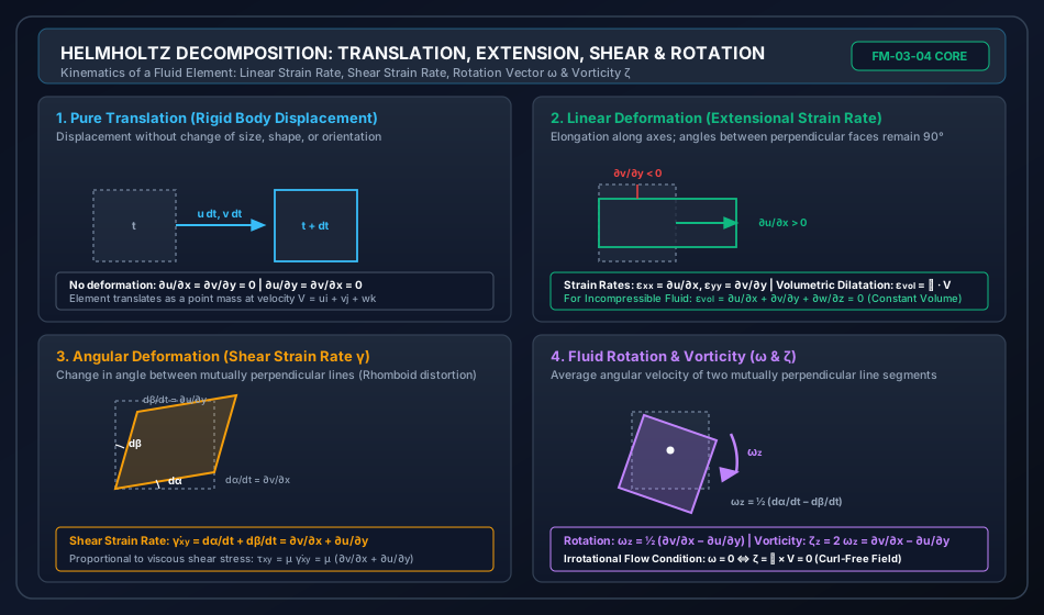
When a rigid solid moves in space, its motion is restricted exclusively to translation and rotation without any internal distortion of its shape. In contrast, an infinitesimal fluid element undergoes continuous deformation under the action of spatial velocity gradients. By the fundamental Helmholtz Decomposition Theorem, the general motion of any fluid parcel over a differential time increment is uniquely decomposable into four distinct kinematic modes:
- Pure Translation: Uniform displacement of the parcel centroid ().
- Linear Deformation (Extensional Strain Rate): Elongation or contraction of edges along coordinate axes (, etc.), resulting in volumetric dilatation ().
- Angular Deformation (Shear Strain Rate): Progressive change in the original angle between mutually orthogonal line segments (). This distortion is directly linked to viscous shear stresses via Newton's law of viscosity ().
- Pure Rotation: Rigid-body angular rotation of the parcel about its centroid without shape distortion, defined as the average angular velocity of two orthogonal intersecting line segments:
The Vorticity Vector is defined mathematically as the curl of the velocity field and is exactly twice the rotation vector:
If throughout a domain, the flow is classified as Irrotational (or potential flow). In civil engineering hydraulics, a vital distinction exists between a Forced Vortex (solid-body rotation induced by external mechanical work, such as a pump impeller, where and ) and a Free Vortex (motion conserving angular momentum, such as water draining into a bottom sluice or bathtub sink, where and everywhere except at the central singular core ).
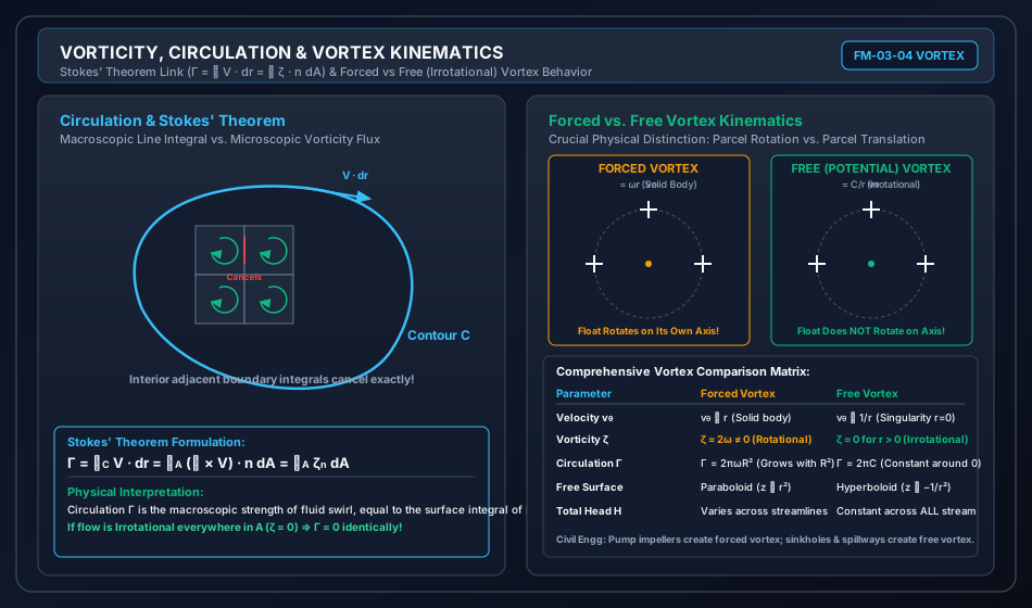
The macroscopic manifestation of fluid swirl is Circulation (), defined as the line integral of velocity around a closed contour: . By Stokes' Theorem, circulation is identically equal to the total net flux of vorticity passing through any open surface bounded by the contour:
In any simply connected irrotational flow field, circulation around every closed path vanishes identically (), forming the mathematical bedrock for velocity potential functions and flow net analysis.
3. General Helmholtz Decomposition of Fluid Motion
Consider an infinitesimal fluid parcel centered at point having velocity . A neighboring point located at has velocity .
Expanding by first-order Taylor series:
In tensor notation, the velocity gradient tensor can be decomposed into a symmetric tensor and an anti-symmetric tensor :
                TOTAL FLUID ELEMENT MOTION (Helmholtz Decomposition)
                                       │
        ┌──────────────────────────────┼──────────────────────────────┐
        ▼                              ▼                              ▼
  TRANSLATION                 STRAIN TENSOR S_ij              SPIN TENSOR Ω_ij
  Displacement of             Rate of Deformation             Rigid-Body Rotation
  parcel centroid             (Shape & Size Change)           (Orientation Change)
  (u dt, v dt, w dt)                   │                               │
                        ┌──────────────┴──────────────┐                ▼
                        ▼                             ▼         Rotation Vector:
                 LINEAR STRAIN                  SHEAR STRAIN    ω = 1/2 (∇ × V)
                 (Extensional)                  (Angular)       Vorticity Vector:
                 ε_xx = ∂u/∂x                   γ_xy = ∂v/∂x    ζ = 2ω = ∇ × V
                 ε_yy = ∂v/∂y                        + ∂u/∂y
                 ε_zz = ∂w/∂z
                 Dilatation: ∇·V
4. Rate of Strain Tensor & Deformation Components
4.1 Linear Strain Rates (Extensional Deformation)
Linear strain rate is defined as the time rate of elongation per unit original length along a coordinate axis:
4.2 Volumetric Dilatation Rate
The volumetric strain rate (rate of change of volume per unit volume) is the trace of the strain rate tensor:
Physical Significance:
- For an incompressible fluid (such as water in civil engineering hydraulic structures), . Although individual fluid parcels may stretch in one direction and compress in another, their volume remains strictly preserved.
4.3 Angular Strain Rate (Shear Deformation)
Consider two initially orthogonal line segments (length , along ) and (length , along ).
- In time , point moves in the -direction relative to by . The counterclockwise angular tilt of segment is:
- In time , point moves in the -direction relative to by . The clockwise angular tilt of segment is:
The Shear Strain Rate () is the rate of decrease of the angle between the two initially perpendicular lines:
In 3D Cartesian coordinates, the complete set of engineering shear strain rates is:
5. Rotation Vector & Vorticity Tensor
5.1 Fluid Rotation Vector ()
Rotation of a fluid element about an axis is defined as the average angular velocity of two mutually perpendicular line segments initially oriented along coordinate axes.
Taking counterclockwise rotation as positive:
- Segment rotates counterclockwise at rate .
- Segment rotates clockwise at rate (which is in the counterclockwise sense).
The average angular velocity about the -axis is:
Similarly, cyclic permutation yields the rotation components about the and axes:
In vector calculus notation:
where the determinant form is:
5.2 Vorticity Vector ()
Vorticity is defined directly as the curl of the velocity vector:
Scalar components of vorticity:
High-Yield Exam Rule:
Students frequently drop the factor of , leading to numerical errors on GATE and ESE.
5.3 Physical Criterion: Rotational vs. Irrotational Flow
- Rotational Flow ( or ): Fluid parcels physically rotate about their own centroids as they travel. A tiny microscopic paddle wheel placed in the flow will spin on its axis. Boundary layers, pipe wall shear zones, hydraulic jumps, and wake separations are strongly rotational.
- Irrotational Flow ( or ): Fluid parcels translate and deform, but their net angular rotation about their centroids is zero (). A tiny paddle wheel will orbit along the streamline without spinning on its axis. External flows away from solid boundaries (ideal potential flow) are irrotational.
6. Circulation & Stokes' Theorem
6.1 Definition of Circulation ()
Circulation is a macroscopic scalar measure of fluid rotation within a finite region. It is defined as the line integral of the tangential velocity component around a closed contour :
where:
- The line integral is traversed in the counterclockwise (positive) direction.
- is the differential displacement along contour .
6.2 Stokes' Theorem Bridge
By Stokes' Theorem of vector calculus, the line integral of any continuous vector field around a closed curve equals the surface integral of its curl over any open surface bounded by :
Substituting :
Physical Meaning: Circulation is the net flux of vorticity passing through the area enclosed by contour .
- If the flow is irrotational everywhere within the domain enclosed by (): Circulation around any closed loop in a simply connected irrotational flow field is identically zero.
7. Kinematic Analysis of Vortices: Forced Vortex vs Free (Potential) Vortex
Vortices are ubiquitous in civil hydraulic engineering, occurring at dam spillway intakes, pump sumps, turbine draft tubes, and river bridge piers.
                           COMPARISON OF VORTEX REGIMES
                                         │
                 ┌───────────────────────┴───────────────────────┐
                 ▼                                               ▼
           FORCED VORTEX                                   FREE VORTEX
      (Solid-Body Rotation)                            (Potential Flow)
                 │                                               │
  v_θ = ω · r                                      v_θ = C / r
  Linear velocity profile                          Hyperbolic velocity profile
  Non-zero vorticity: ζ = 2ω                       Zero vorticity: ζ = 0 (for r > 0)
  Rotational Flow (Paddle wheel spins)             Irrotational Flow (Float does not spin)
  Free surface: Paraboloid (z ∝ r²)                Free surface: Hyperboloid (z ∝ -1/r²)
  Total energy head varies across r                Total energy head constant everywhere
  Example: Centrifugal pump impeller               Example: Bathtub drain, spillway intake
Detailed Kinematic Comparison Matrix
| Parameter / Feature | Forced Vortex (Solid-Body Rotation) | Free (Potential / Irrotational) Vortex |
|---|---|---|
| Governing Tangential Velocity | (where ) | |
| Radial Velocity () | (or inward sink ) | |
| Vorticity () | ||
| Flow Classification | Rotational Flow | Irrotational Flow (except singularity at ) |
| Motion of a Floating Cross | Float rotates on its own axis as it orbits | Float translates in orbit; arms retain constant orientation |
| Circulation (Radius , enclosing origin) | (Grows with ) | |
| Circulation (Loop NOT enclosing origin) | ||
| Free Surface Profile | Paraboloid of revolution: | Hyperbolic depression: |
| Total Mechanical Energy Head () | Varies radially: (Torque input required) | Strictly constant across all streamlines: (Euler-Bernoulli equation holds globally) |
| Civil Engineering Example | Liquid in a rotating vessel; centrifugal pump impeller; vertical turbine runner | Water draining from bottom orifice; whirlpool at spillway inlet; cyclonic dust devil |
8. Visual Diagrams & Architectural Schematics
8.1 Helmholtz Decomposition of Fluid Element Motion
The schematic below visualizes the four fundamental modes of continuum fluid motion: pure translation, linear extensional deformation, angular shear distortion, and rigid-body rotation.
8.2 Vorticity, Circulation, Stokes' Theorem & Vortex Regimes
The diagram below presents the equivalence between microscopic vorticity flux and macroscopic contour circulation via Stokes' Theorem, alongside the comparative kinematics of forced versus free vortices.
9. Step-by-Step Numerical Problems with Complete Calculations
Problem 1: 2D Deformation Tensor & Irrotationality Check
Problem Statement: A two-dimensional incompressible fluid flow field is given by:
At the spatial coordinate :
- Compute the linear strain rates and .
- Verify whether the flow satisfies the incompressible continuity equation ().
- Compute the engineering shear strain rate .
- Compute the fluid rotation rate and vorticity . State whether the flow is rotational or irrotational.
Step 1: Compute Partial Velocity Derivatives
At point :
Step 2: Linear Strain Rates & Incompressibility Check
The volumetric dilatation rate is:
Conclusion: The volumetric dilatation rate is identically zero. The fluid flow is incompressible.
Step 3: Compute Shear Strain Rate
The negative sign indicates that the angle between lines initially parallel to the and axes is increasing at a rate of .
Step 4: Compute Rotation and Vorticity
Conclusion: Since both rotation and vorticity vanish identically, the flow field is irrotational.
Problem 2: Laminar Couette Shear Flow & Stokes' Theorem Verification
Problem Statement: In steady laminar Couette flow between two wide horizontal parallel plates separated by clearance , the lower plate is stationary () while the upper plate () moves steadily at velocity . The velocity profile is linear:
- Determine the shear strain rate , fluid rotation rate , and vorticity .
- Compute the circulation around a closed rectangular loop of length in the -direction and height in the -direction, oriented counterclockwise with vertices at : a) By direct line integration: . b) By surface area integration using Stokes' Theorem: . Verify that both results match identically.
Step 1: Kinematic Deformation Rates
Velocity components:
Partial derivatives:
- Shear strain rate:
- Rotation rate: (Clockwise rotation of fluid elements).
- Vorticity:
Step 2: Circulation via Direct Line Integration
Decompose contour into four straight segments:
- Segment 1 (Bottom Edge: , from to ):
- Segment 2 (Right Edge: , from to ):
- Segment 3 (Top Edge: , from to ):
- Segment 4 (Left Edge: , from to ):
Summing all four edges:
Step 3: Circulation via Stokes' Theorem Surface Integral
Since the vorticity is uniform across the entire rectangle:
Verification: . The results match with zero discrepancy.
Problem 3: Forced Vortex vs Free Vortex Vorticity & Circulation
Problem Statement: Compare the kinematic circulation and vorticity characteristics of two cylindrical swirling flows:
- Forced Vortex: A cylinder containing water rotates as a rigid body about its vertical axis at an angular velocity of . The tangential velocity is .
- Calculate the vorticity at radius .
- Compute the circulation around a circular path of radius centered at the axis.
- Free (Potential) Vortex: Water drains freely into a bottom outlet with a tangential velocity field given by , where .
- Calculate the vorticity at any radius .
- Compute the circulation around a circular path of radius centered at the origin.
- Compute the circulation around a square contour of side situated entirely in the region (not enclosing the origin).
Step 1: Forced Vortex Kinematics
Tangential velocity: . In cylindrical coordinates, the -component of vorticity is:
Since :
Circulation around circle of radius :
Alternatively by Stokes' Theorem:
Step 2: Free Vortex Kinematics
Tangential velocity: . Vorticity for any :
Conclusion: The free vortex has zero vorticity everywhere outside the singular origin . The flow is irrotational.
Circulation around circle of radius enclosing the origin:
Notice that is completely independent of the radius ! Any contour enclosing the origin yields the exact same circulation .
Circulation around contour NOT enclosing the origin: Since the region is simply connected and throughout:
10. High-Yield Exam Pitfalls, Traps & Shortcuts
- The Circular Streamlines Rotational Flow Trap:
- Common Myth: "If streamlines are curved or circular, the flow must be rotational."
- Reality: Circular streamlines can be entirely irrotational! A Free Vortex has concentric circular streamlines, yet its vorticity is identically zero everywhere ( for ). Rotation depends on whether fluid parcels twist on their own centroids, NOT on whether their path of translation is curved.
- Factor of 2 Confusion between Vorticity and Rotation:
- Always remember:
- If asked for rotation (): use .
- If asked for vorticity (): use .
- Always remember:
- Boundary Layer Vorticity Generation:
- Real fluids have viscosity (). By the no-slip condition at solid walls ( at ), severe velocity gradients are created, making boundary layers intensely rotational (). Vorticity is continuously generated at solid boundaries and diffuses into the flow.
- Stokes' Theorem Singularity Catch:
- Stokes' theorem states . If a contour encloses a point singularity (such as the central filament of a free vortex), you cannot naively set just because elsewhere. The singularity acts as a concentrated line vortex carrying circulation .
- Quick Shortcut for Determining Irrotationality:
- Given :
- If equal: Irrotational ().
- If unequal: Rotational ().
- Given :
11. Multi-Exam Question Bank (GATE, ESE, SSC JE, State AE, RRB JE)
Question 1 (GATE CE — Analytical)
The velocity field in a fluid is given by . The vorticity vector at the point is:
(A)
(B)
(C)
(D)
Solution: Here, and . Compute spatial cross-derivatives:
Vorticity :
At the point :
(Note: If asked for rotation component , it would be ). Correct Option: (D)
Question 2 (UPSC ESE Paper-II — Descriptive / Analytical)
Consider the following statements regarding a free vortex and a forced vortex:
- In a forced vortex, velocity is directly proportional to radius ().
- In a free vortex, vorticity is non-zero everywhere.
- The circulation around a closed circuit enclosing the center of a free vortex is independent of the circuit radius.
- Total mechanical energy head is constant across all streamlines in a forced vortex.
Which of the above statements are CORRECT?
(A) 1 and 3 only
(B) 1, 2, and 3
(C) 2 and 4 only
(D) 1, 3, and 4
Solution:
- Statement 1 is correct: in a forced vortex.
- Statement 2 is incorrect: In a free vortex, vorticity for all (it is irrotational).
- Statement 3 is correct: , independent of .
- Statement 4 is incorrect: In a forced vortex, external torque does work, causing total head to increase with radius (). It is in a free vortex that is constant across all streamlines.
Therefore, only statements 1 and 3 are correct.
Correct Option: (A)
Question 3 (SSC JE — Direct Conceptual)
The vorticity of a fluid flow field is:
(A) Equal to the angular velocity
(B) Equal to half of the angular velocity
(C) Equal to twice the angular velocity
(D) Equal to the square of the angular velocity
Solution:
Vorticity is defined as . It is twice the angular velocity (rotation vector) of the fluid parcel.
Correct Option: (C)
Question 4 (State PSC AE — Numerical)
In a two-dimensional flow, the velocity components are and . The rotation of the fluid parcel about the -axis is:
(A)
(B)
(C)
(D)
Solution: Here, . . Rotation about -axis:
The flow is completely irrotational.
Correct Option: (A)
Question 5 (RRB JE — Direct Knowledge)
Stokes' Theorem connects:
(A) A line integral around a closed curve to a volume integral
(B) A surface integral over a closed surface to a volume integral
(C) A line integral around a closed curve to a surface integral over an open surface
(D) A point value to a line integral
Solution:
Stokes' Theorem relates the line integral of a vector field around a closed boundary curve to the surface integral of the curl of that vector field over an open surface bounded by : . (Gauss Divergence theorem connects closed surface integrals to volume integrals).
Correct Option: (C)
12. Comprehensive Summary, Formula Cheatsheet & Academic References
12.1 Formula Cheatsheet
┌────────────────────────────────────────────────────────────────────────────────────────┐
│                        FLUID DEFORMATION & VORTEX CHEATSHEET                           │
├────────────────────────────────────────────────────────────────────────────────────────┤
│ 1. Rate of Strain Components (Cartesian):                                              │
│    Linear:    ε_xx = ∂u/∂x,   ε_yy = ∂v/∂y,   ε_zz = ∂w/∂z                             │
│    Dilatation: ε_vol = ∇·V = ε_xx + ε_yy + ε_zz (= 0 for Incompressible Flow)          │
│    Shear:     γ_xy = ∂v/∂x + ∂u/∂y,  γ_yz = ∂w/∂y + ∂v/∂z,  γ_zx = ∂u/∂z + ∂w/∂x       │
│                                                                                        │
│ 2. Fluid Rotation Vector (ω):                                                          │
│    ω = 1/2 (∇ × V) = ωx i + ωy j + ωz k                                                │
│    ωz = 1/2 (∂v/∂x - ∂u/∂y),  ωx = 1/2 (∂w/∂y - ∂v/∂z),  ωy = 1/2 (∂u/∂z - ∂w/∂x)      │
│                                                                                        │
│ 3. Vorticity Vector (ζ):                                                               │
│    ζ = ∇ × V = 2ω                                                                      │
│    ζz = 2ωz = ∂v/∂x - ∂u/∂y                                                            │
│    Irrotational Flow Condition: ζ = 0 <=> ω = 0 <=> ∇ × V = 0                          │
│                                                                                        │
│ 4. Circulation (Γ) & Stokes' Theorem:                                                  │
│    Γ = ∮_C V·dr = ∬_A (∇ × V)·n dA = ∬_A ζ·n dA = 2 ∬_A ω_n dA                         │
│    For Irrotational Simply-Connected Flow: Γ = 0 identically                           │
│                                                                                        │
│ 5. Vortex Kinematics Summary:                                                          │
│    Forced Vortex: v_θ = ωr,     ζ = 2ω (Rotational),  Γ = 2πωR²,  z = ω²r²/(2g)        │
│    Free Vortex:   v_θ = C/r,    ζ = 0 (Irrotational), Γ = 2πC,    z = -C²/(2gr²)       │
└────────────────────────────────────────────────────────────────────────────────────────┘
12.2 Academic & Standard References
- White, F. M. (2016). Fluid Mechanics (8th ed.). McGraw-Hill Education, New York. (Chapter 4: Differential Relations for Fluid Flow — Deformation, Rotation, and Vorticity).
- Kundu, P. K., Cohen, I. M., & Dowling, D. R. (2016). Fluid Mechanics (6th ed.). Academic Press / Elsevier. (Chapter 3: Kinematics and Vorticity Dynamics).
- Fox, R. W., McDonald, A. T., & Pritchard, P. J. (2015). Introduction to Fluid Mechanics (9th ed.). John Wiley & Sons.
- Modi, P. N., & Seth, S. M. (2018). Hydraulics and Fluid Mechanics Including Hydraulics Machines (22nd ed.). Standard Book House, New Delhi. (Chapter 5: Fluid Kinematics — Vorticity and Circulation).
- Bureau of Indian Standards. IS 1192: Velocity-Area Methods for Measurement of Flow of Water in Open Channels. New Delhi, India.