Bernoulli Applications: Venturimeter, Orifice Meter & Pitot-Static Tube
In this chapter (4 topics)
On this page
- 1. Topic Metadata Table
- 2. Executive Summary
- 3. Venturimeter Mechanics, Flow Equations & Diffuser Design Criteria
- 3.1 Structural Components & Geometric Ratios
- 3.2 Formal Derivation of Venturimeter Discharge Equation
- 4. Orifice Meter (Orifice Plate), Vena Contracta & Hydraulic Coefficients
- 4.1 Construction & Vena Contracta Formation
- 4.2 The Three Fundamental Hydraulic Coefficients
- 4.3 Orifice Meter Discharge Equation
- 4.4 Pressure Tapping Configurations (IS 2951 / ISO 5167)
- 5. Head Loss Comparison: Venturimeter vs Orifice Meter & Economic Life-Cycle Considerations
- 6. Pitot Tube & Prandtl Pitot-Static Tube: Stagnation Pressure & Flow Velocity Measurement
- 6.1 Operating Physics & Stagnation State
- 6.2 The Simple Pitot Tube in an Open Channel
- 6.3 The Prandtl Pitot-Static Tube in Closed Conduits
- 7. Manometer Fluid Deflection Equations for Differential Flow Meters
- 7.1 Case 1: Manometric Liquid is Heavier than Flowing Liquid (Sm > S)
- 7.2 Case 2: Manometric Liquid is Lighter than Flowing Liquid (Sm < S)
- 7.3 Independence of Manometer Reading from Pipeline Orientation
- 8. Visual Diagrams & Hydraulic Schematics
- 8.1 Venturimeter Construction, Manometer & EGL/HGL Profile
- 8.2 Orifice Meter Vena Contracta & Prandtl Pitot-Static Tube
- 9. Step-by-Step Numerical Problems with Complete Calculations
- Problem 1: Inclined Venturimeter with Mercury Manometer (Orientation & Head)
- Problem 2: Orifice Meter vs Venturimeter Comparative Energy Loss & Lifetime Pumping Cost
- Problem 3: Prandtl Pitot-Static Tube Air Velocity in Wind Tunnel Duct
- 10. High-Yield Exam Pitfalls, Traps & Shortcuts
- 11. Multi-Exam Question Bank (GATE, ESE, SSC JE, State AE, RRB JE)
- Question 1 (GATE CE — Multiple Choice Question)
- Question 2 (UPSC ESE Paper-II)
- Question 3 (SSC JE)
- Question 4 (State PSC AE)
- Question 5 (RRB JE)
- 12. Comprehensive Summary, Formula Cheatsheet & Academic References
- Master Formula Cheatsheet
- Academic References & Standard Source Texts
1. Topic Metadata Table
| Field | Detail |
|---|---|
| Subject | Fluid Mechanics & Hydraulic Machinery (Subject 07) |
| Chapter | Chapter 04: Fluid Dynamics & Momentum Equation |
| Topic Code | FM-04-02 |
| Topic Title | Practical Applications of Bernoulli's Theorem: Venturimeter (Convergent-Divergent Cone, Throat Sizing, ), Orifice Meter (Vena Contracta, ), Pitot Tube & Prandtl Pitot-Static Tube (Stagnation Dynamics) |
| Prerequisites | FM-04-01 (Euler's & Bernoulli's Equations, EGL/HGL), FM-02-01 & FM-02-02 (Hydrostatics & U-Tube Manometry), FM-03-02 (Continuity Equation) |
| Target Examinations | GATE CE, UPSC ESE (Paper-II), SSC JE, State PSC AE/JE, RRB JE |
| Knowledge Level | Comprehensive Closed-Conduit Flow Measurement to Practical Field Hydraulics |
| IS / ISO / Standard Codes | IS 2951 (Part 1 & 2: Measurement of fluid flow in closed conduits by means of orifice plates and nozzles), ISO 5167 (Measurement of fluid flow by means of pressure differential devices inserted in circular cross-section conduits running full), ASME MFC-3M |
| Key Formulae | , , , , , |
2. Executive Summary
Bernoulli’s principle of mechanical energy conservation along a streamline provides the foundational operating physics for the primary differential-pressure flowmeters utilized in civil, environmental, water-supply, and irrigation engineering. By inducing a localized fluid acceleration through a known geometric constriction, static pressure is converted into dynamic velocity head; measuring the resulting piezometric pressure drop () enables direct determination of volumetric flow rate () or local velocity ().
Three primary flow-measurement instruments dominate technical practice:
- The Venturimeter:
- A streamlined closed-conduit meter comprising a short convergent cone (), a cylindrical throat (), and an extended, gradual divergent cone (diffuser, ).
- The gradual divergent angle strictly prevents adverse pressure gradient boundary-layer separation and wake stall, resulting in an exceptionally high coefficient of discharge () and an exceptionally low permanent head loss ( of measured differential head ).
- Theoretical discharge:
- Crucially, the measured piezometric head difference is completely invariant to the physical inclination of the meter (horizontal, vertical, or angled).
- The Orifice Meter (Orifice Plate):
- A thin circular flat plate with a sharp, square-edged concentric aperture () clamped between pipeline flanges.
- Fluid inertia prevents the streamlines from executing a sharp turn, forcing the issuing jet to continue converging downstream of the plate until it reaches its minimum cross-sectional area, termed the Vena Contracta (), located at approximately downstream.
- Governed by three hydraulic coefficients: Coefficient of Contraction (), Coefficient of Velocity (), and Coefficient of Discharge ().
- While physically compact, inexpensive, and easy to service, the sudden expansion downstream of the vena contracta generates severe turbulent eddy dissipation, imposing a permanent energy loss of of .
- The Pitot Tube & Prandtl Pitot-Static Tube:
- Employs a forward-facing impact orifice aligned along the local streamline to bring fluid particles to a complete rest () at a Stagnation Point.
- The pressure measured at the impact opening is the Stagnation / Total Pressure:
- By integrating circumferential wall taps on an outer concentric sleeve, the Prandtl Pitot-Static Tube measures static pressure () simultaneously, isolating the dynamic pressure to yield local velocity: with .
3. Venturimeter Mechanics, Flow Equations & Diffuser Design Criteria
3.1 Structural Components & Geometric Ratios
A standard classical Herschel venturimeter consists of three contiguous geometric zones:
- Converging Section (Entrance Cone):
- A truncated cone that contracts the flow from pipe diameter down to throat diameter .
- Included angle: .
- Flow accelerates under a favorable pressure gradient (); hence, the boundary layer remains thin, stable, and completely attached. Friction loss in this zone is virtually negligible.
- Throat Section:
- A short, true cylindrical section of uniform diameter and length .
- Typical diameter ratio: (or per IS 2951).
- The velocity reaches its maximum (), producing minimum static pressure ().
- Diverging Section (Diffuser):
- An elongated truncated cone expanding from back to the original pipe diameter .
- Included angle: (never exceeding ).
- Why is the diverging cone significantly longer than the converging cone? In the diverging section, flow decelerates, causing static pressure to rise in the direction of flow (, an Adverse Pressure Gradient). If the expansion angle exceeds , fluid particles near the wall within the viscous boundary layer run out of kinetic energy, decelerate to zero, and reverse direction. This precipitates Boundary Layer Separation, generating large-scale recirculating eddies, turbulent wake stall, and severe permanent dissipation of mechanical energy into heat. By keeping restricted to , flow remains fully attached, maximizing static pressure recovery.
       <-- Convergent -->|< Throat >|<--------- Divergent Cone (Diffuser) --------->
                         |          |
Pipe Wall ===============\          /================================ Pipe Wall
                          \________/
Centerline - - - - - - - - - - - - - - - - - - - - - - - - - - - - - - - - - - - -
                          /¯¯¯¯¯¯¯¯\
Pipe Wall ===============/          \================================ Pipe Wall
       Angle: 20° - 22°              Angle: 5° - 7° (Elongated to prevent separation)
3.2 Formal Derivation of Venturimeter Discharge Equation
Consider steady, incompressible flow of an ideal fluid between inlet Section 1 () and throat Section 2 ().
Step 1: Continuity Equation
Step 2: Ideal Bernoulli Equation
Group piezometric heads:
Let the differential piezometric head be:
Then:
Step 3: Solve for Throat Velocity
Substitute :
Step 4: Theoretical Discharge ()
Introducing the area ratio (diameter ratio where ):
The dimensionless term is known as the Velocity of Approach Factor.
Step 5: Actual Discharge () and Coefficient of Discharge ()
Real fluids experience slight boundary-layer skin friction and non-uniform velocity distribution between inlet and throat:
where:
- (Coefficient of Discharge): (For high pipe Reynolds numbers , approaches to . It depends mildly on Reynolds number and surface roughness, but is essentially constant in fully turbulent flow).
4. Orifice Meter (Orifice Plate), Vena Contracta & Hydraulic Coefficients
4.1 Construction & Vena Contracta Formation
An Orifice Meter consists of a flat, circular metal plate (typically stainless steel or bronze) with a concentric circular hole of diameter , machined with a sharp upstream edge ( bevel). It is clamped perpendicularly between two standard pipe flanges.
Pipe Wall =================[|]================================ Pipe Wall
                            |
Flow --->   - - - - - - - - \   ) ) )  Vena Contracta
            - - - - - - - - - > ) ) )   a_c < a_0
            - - - - - - - - /   ) ) )  (Sec 2)
                            |
Pipe Wall =================[|]================================ Pipe Wall
                         Orifice Plate (d_0)
Because of fluid momentum, streamlines converging toward the opening cannot make an abrupt right-angled turn at the sharp edge. Instead, the jet continues to contract downstream of the orifice until the streamlines become completely parallel and the jet reaches its minimum cross-sectional area.
- This section of minimum jet area is called the Vena Contracta (Section 2).
- The vena contracta is located at a distance of approximately (nominally ) downstream of the orifice plate.
- At the vena contracta:
- Velocity is maximum ().
- Pressure is minimum ().
- Streamlines are straight and parallel; thus, the pressure distribution across the jet is purely hydrostatic.
4.2 The Three Fundamental Hydraulic Coefficients
- Coefficient of Contraction (): The ratio of the cross-sectional area of the jet at the vena contracta () to the geometric area of the orifice aperture (): Typical values: . (For a sharp circular Borda mouthpiece or free orifice, ).
- Coefficient of Velocity (): The ratio of the actual jet velocity at the vena contracta () to the ideal frictionless theoretical velocity (): Typical values: (very close to unity because friction loss up to the vena contracta is minimal).
- Coefficient of Discharge (): The ratio of the actual discharge to the ideal theoretical discharge: Typical values: (frequently taken as in standard calculations).
4.3 Orifice Meter Discharge Equation
Applying Bernoulli's theorem between pipe inlet Section 1 () and the vena contracta Section (), the discharge through the orifice meter is:
4.4 Pressure Tapping Configurations (IS 2951 / ISO 5167)
Because the vena contracta location varies slightly with Reynolds number and diameter ratio , standardized pressure taps are used:
- Corner Taps: Tappings located directly in the corner formed by the pipe wall and the orifice plate face. Common for small pipes ().
- Flange Taps: Tappings drilled through the pipe flanges exactly () upstream and downstream from the plate faces. Most popular in industrial pipeline installations.
- and Taps (Radius Taps): Upstream tap located at distance from the plate; downstream tap located at distance (coinciding with the vena contracta).
5. Head Loss Comparison: Venturimeter vs Orifice Meter & Economic Life-Cycle Considerations
While both meters operate on the same differential pressure principle, their fluid mechanical efficiency and economic profiles diverge drastically:
| Feature / Criterion | Venturimeter | Orifice Meter (Plate) |
|---|---|---|
| Coefficient of Discharge () | (Very high, streamlined) | (Jet contraction) |
| Permanent Head Loss () | Low: of differential head | High: of differential head |
| Physical Mechanism of Loss | Gradual wall friction in diffuser cone; separation suppressed by | Sudden expansion downstream of vena contracta; violent eddy shedding |
| Capital & Installation Cost | Very high (precision casting, machined cone, large footprint) | Very low (simple machined plate clamped between flanges) |
| Space Requirements | Large length required () | Negligible axial length ( plate thickness) |
| Susceptibility to Wear & Clogging | Low (smooth contours resist erosion and suspended sediment) | High (sharp edge rounds over time from abrasion, altering ) |
| Operational Pumping Cost | Minimal continuous energy dissipation | Very high continuous pumping cost over plant lifetime |
Permanent Head Loss Comparison:
Differential Head Delta h ========================================== (100%)
Venturimeter Loss         [====] (10 - 15%)
Orifice Meter Loss        [============================] (60 - 75%)
Economic Engineering Rule: For continuous pumping systems (such as municipal water distribution, high-pressure feedwater lines, and crude oil pipelines operating 8,760 hours/year), the extra capital expenditure of a Venturimeter is amortized within months through electrical power savings, rendering the orifice meter economically unfeasible despite its cheaper initial price!
6. Pitot Tube & Prandtl Pitot-Static Tube: Stagnation Pressure & Flow Velocity Measurement
6.1 Operating Physics & Stagnation State
A Pitot Tube is an L-shaped open-ended glass or metal tube bent at and inserted into a flowing stream with its open tip pointing directly into the oncoming velocity vector.
When a moving fluid particle approaches the open mouth along the central streamline, it is forced to decelerate to a complete stop at the mouth.
- A point in a flow field where the fluid velocity is brought to rest is called a Stagnation Point ().
- Applying Bernoulli's equation between an undisturbed upstream point 1 () and the stagnation point 0 ():
Multiplying throughout by :
where:
- : Static Pressure (actual thermodynamic pressure exerted by fluid particles on surfaces parallel to flow),
- : Dynamic Pressure (kinetic energy per unit volume),
- : Stagnation Pressure (Total Pressure) (pressure achieved when dynamic pressure is converted isentropically into static pressure).
6.2 The Simple Pitot Tube in an Open Channel
In an open-channel flow where surface static pressure is hydrostatic (, depth of immersion):
- Fluid rises in the vertical leg of the tube to a height above the channel bed:
- The rise of liquid inside the tube above the surrounding free surface is directly the velocity head:
- Actual local streamline velocity: where is the Pitot tube velocity coefficient.
6.3 The Prandtl Pitot-Static Tube in Closed Conduits
In a pressurized pipe or air duct, measuring static pressure requires a separate wall piezometer or a dual concentric tube design. The Prandtl Pitot-Static Tube combines both sensors into a single aerodynamic probe:
- Inner Central Tube: Faces oncoming flow to sense Stagnation Pressure ().
- Outer Concentric Annular Sleeve: Contains tiny circumferential holes drilled perpendicular to the flow at a distance tube diameters downstream of the nose tip. These holes sense undisturbed Static Pressure ().
- Differential Manometer Connection: Connecting the inner and outer tube taps to a differential U-tube manometer measures dynamic pressure directly:
When connected to a manometer containing manometric liquid of density showing deflection :
7. Manometer Fluid Deflection Equations for Differential Flow Meters
When a differential U-tube manometer is connected across the inlet and throat of a venturimeter, orifice meter, or nozzle, the deflection of the manometric liquid meniscus is designated by .
7.1 Case 1: Manometric Liquid is Heavier than Flowing Liquid ()
Example: Water or oil flowing in pipe (), Mercury in manometer (). Equating pressures at the horizontal datum of the lower meniscus in the U-tube:
Therefore, the differential piezometric head is:
7.2 Case 2: Manometric Liquid is Lighter than Flowing Liquid ()
Used for measuring small pressure differences (Inverted U-Tube Manometer with light oil or air over water):
7.3 Independence of Manometer Reading from Pipeline Orientation
CRITICAL GATE / ESE PRINCIPLE: The relationship holds identically whether the venturimeter is:
- Horizontal (),
- Inclined Upwards (),
- Inclined Downwards (), or
- Vertical ().
Reason: The U-tube manometer measures the difference in piezometric head , NOT just static pressure difference . The elevation difference between the pressure taps is automatically compensated by the liquid columns in the manometer lead tubes!
8. Visual Diagrams & Hydraulic Schematics
8.1 Venturimeter Construction, Manometer & EGL/HGL Profile
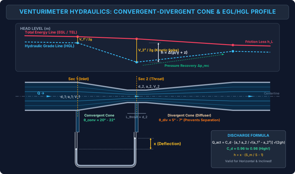
The schematic below details the geometry of a Herschel venturimeter, illustrating the convergent cone, cylindrical throat, diffuser cone, mercury U-tube manometer, and the corresponding profiles of the Energy Grade Line (EGL) and Hydraulic Grade Line (HGL).
8.2 Orifice Meter Vena Contracta & Prandtl Pitot-Static Tube
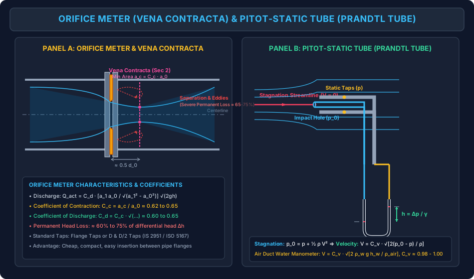
The multi-panel diagram below contrasts the flow dynamics of an Orifice Meter (vena contracta, contraction coefficient , recirculating separation eddies, and permanent head loss) against the stagnation physics of a Prandtl Pitot-Static Tube.
9. Step-by-Step Numerical Problems with Complete Calculations
Problem 1: Inclined Venturimeter with Mercury Manometer (Orientation & Head)
Problem Statement: An inclined venturimeter is installed in an oil pipeline carrying oil of specific gravity (). The pipeline slopes upwards at an angle to the horizontal.
- Inlet diameter: .
- Throat diameter: .
- Distance along the pipe axis between inlet and throat pressure taps: .
- A differential U-tube mercury manometer () connected across the taps records a meniscus deflection .
- Discharge coefficient of the venturimeter: .
- Acceleration due to gravity: .
Determine:
- Differential piezometric head in meters of oil,
- Theoretical discharge and actual discharge in ,
- Elevation difference ,
- Static pressure difference in .
Solution & Step-by-Step Calculation:
Step 1: Compute cross-sectional flow areas
Step 2: Differential piezometric head ()
Step 3: Theoretical and Actual Discharge
Actual discharge:
Step 4: Elevation difference between sections
Step 5: Static pressure difference By definition of piezometric head difference:
Rearranging for static pressure difference:
Problem 2: Orifice Meter vs Venturimeter Comparative Energy Loss & Lifetime Pumping Cost
Problem Statement: A municipal water transmission main of diameter () delivers water () at a volumetric flow rate ().
- A standard sharp-edged concentric orifice plate with hole diameter () and is installed. Calculate the differential head in meters of water and the reading on a mercury manometer ().
- If the permanent head loss caused by the orifice meter is of the differential head, while a comparable venturimeter would cause a permanent head loss of only of the differential head, calculate the extra hydraulic power dissipated by the orifice meter.
- If the pipeline operates continuously () and pumping power is supplied by an electrically driven pump of overall efficiency at an electricity tariff of ₹, compute the annual financial loss resulting from choosing the orifice plate over the venturimeter.
Solution & Step-by-Step Calculation:
Step 1: Compute geometric areas and velocity of approach factor
Step 2: Compute differential head
Manometer deflection :
Step 3: Head losses and extra power dissipated
Extra Electrical Power Consumed ():
Step 4: Annual Energy and Financial Cost
Civil Engineering Conclusion: Even for a modest line pumping , the orifice meter wastes over ₹2.09 Lakhs every single year in electric power. A venturimeter pays for its extra fabrication cost in under 6 to 9 months!
Problem 3: Prandtl Pitot-Static Tube Air Velocity in Wind Tunnel Duct
Problem Statement: A Prandtl Pitot-static tube () is placed along the centerline of a circular air duct of diameter conveying atmospheric air at and ().
- The pressure differential between the stagnation tip and the static wall taps is connected to an inclined water manometer containing water ().
- The manometer tube is inclined at an angle to the horizontal, and the length of the meniscus deflection along the inclined glass scale is .
- The velocity profile across the duct is fully turbulent, following the 1/7th power law where average duct velocity is .
Determine:
- Differential static-to-stagnation pressure in ,
- Centerline maximum flow velocity in ,
- Mean duct velocity in ,
- Total mass flow rate of air through the duct in .
Solution & Step-by-Step Calculation:
Step 1: Vertical water column deflection () and Dynamic Pressure ()
Dynamic pressure:
Step 2: Equivalent air head () and Centerline Velocity ()
Centerline velocity:
Step 3: Mean velocity across the circular duct For turbulent 1/7th power law flow:
Step 4: Cross-sectional duct area and mass flow rate
10. High-Yield Exam Pitfalls, Traps & Shortcuts
-
The "Inclined Venturimeter Orientation" Trap (GATE & ESE):
- Trap: A student calculates using manometer deflection , then adds or subtracts when finding discharge .
- Truth: Do NOT modify ! The differential piezometric head already fully accounts for . Discharge depends purely on : Orientation matters ONLY when explicitly computing the static pressure difference: .
-
Divergent Cone Angle Limit (SSC JE & State AE):
- Trap: Thinking the convergent cone angle must be smaller to avoid losses.
- Truth: The Convergent Cone is short and steep () because flow accelerates (, favorable gradient, no separation).
- The Divergent Cone must be long and gentle () because flow decelerates (, adverse gradient, separation risk).
-
Coefficient Hierarchy ():
- Always remember: .
- For an orifice: , , .
-
Dynamic Pressure vs Stagnation Pressure:
- Static pressure:
- Dynamic pressure:
- Stagnation pressure:
- Stagnation head:
- Pitot tube measures ; Pitot-static tube measures .
-
Inverted Manometer Deflection:
- When a lighter manometric liquid is used: . Do not use or will be negative!
11. Multi-Exam Question Bank (GATE, ESE, SSC JE, State AE, RRB JE)
Question 1 (GATE CE — Multiple Choice Question)
A horizontal venturimeter with inlet diameter and throat diameter is used to measure the flow of water. The pressure at the inlet is and the vacuum pressure at the throat is . If and , the actual discharge through the venturimeter is:
- A)
- B)
- C)
- D)
Detailed Solution: Inlet gauge pressure: . Throat vacuum pressure: . Horizontal meter . Differential piezometric head:
Areas:
Matching option B (). Correct Answer: B
Question 2 (UPSC ESE Paper-II)
Assertion (A): The divergent cone of a venturimeter is made much longer than the convergent cone with an included angle restricted to about .
Reason (R): In the divergent cone, flow takes place under a favorable pressure gradient which accelerates the fluid particles and prevents cavitation.
- A) Both A and R are true, and R is the correct explanation of A
- B) Both A and R are true, but R is not the correct explanation of A
- C) A is true, but R is false
- D) A is false, but R is true
Detailed Solution:
- Assertion (A) is True: The divergent cone is elongated with an angle of .
- Reason (R) is False: In the divergent cone, the cross-sectional area increases, causing velocity to decrease and static pressure to increase (). This is an adverse pressure gradient, NOT a favorable pressure gradient. Fluid particles decelerate, risking boundary-layer separation and eddy loss, which is why the angle is kept so small. Correct Answer: C
Question 3 (SSC JE)
The vena contracta of an orifice in a pipe is located approximately at a distance of:
- A) downstream
- B) downstream
- C) upstream
- D) Exactly at the plane of the orifice plate
Detailed Solution: The streamlines continue converging after passing through the sharp orifice edge and reach minimum cross-sectional area at approximately half the orifice diameter () downstream. Correct Answer: B
Question 4 (State PSC AE)
A Pitot-static tube is used to measure the velocity of water in a pipe. The stagnation pressure head is and the static pressure head is . Taking and coefficient , the velocity of water is:
- A)
- B)
- C)
- D)
Detailed Solution: Dynamic pressure head .
Correct Answer: A
Question 5 (RRB JE)
The relation between the coefficient of discharge (), coefficient of contraction (), and coefficient of velocity () for an orifice is:
- A)
- B)
- C)
- D)
Detailed Solution: By definition, . Correct Answer: C
12. Comprehensive Summary, Formula Cheatsheet & Academic References
Master Formula Cheatsheet
Academic References & Standard Source Texts
- White, F. M. (2016). Fluid Mechanics (8th ed.). McGraw-Hill Education. Chapter 6: Viscous Flow in Ducts (Section 6.12: Flowmeters).
- Modi, P. N., & Seth, S. M. (2018). Hydraulics and Fluid Mechanics Including Hydraulics Machines (22nd ed.). Standard Book House, New Delhi. Chapter 7: Measurement of Flow (Venturimeters, Orifices & Pitot Tubes).
- Streeter, V. L., Wylie, E. B., & Bedford, K. W. (1998). Fluid Mechanics (9th ed.). WCB/McGraw-Hill. Chapter 8: Closed-Conduit Flow.
- Rajput, R. K. (2020). A Textbook of Fluid Mechanics and Hydraulic Machines (7th ed.). S. Chand & Company Ltd. Chapter 6: Dynamics of Fluid Flow.
- IS 2951 (Part 1): Methods of Measurement of Fluid Flow by Means of Venturi Meters. Bureau of Indian Standards, New Delhi.
- ISO 5167-1 & 5167-2: Measurement of fluid flow by means of pressure differential devices inserted in circular cross-section conduits running full - Part 2: Orifice plates.