Lagrangian & Eulerian Descriptions, Flow Classification, Streamlines & Pathlines
In this chapter (5 topics)
On this page
- 1. Topic Metadata & Syllabus Mapping
- 2. Executive Summary & Core Engineering Concepts
- 3. Descriptions of Fluid Motion: Lagrangian vs Eulerian
- 3.1 The Lagrangian Description
- 3.2 The Eulerian Description
- 3.3 The Material (Substantial) Derivative Link
- 4. Comprehensive Taxonomy & Classification of Fluid Flows
- 4.1 Steady vs Unsteady Flow
- 4.2 Uniform vs Non-Uniform Flow
- 4.3 The 4-Quadrant Flow Regime Matrix
- 4.4 Laminar vs Turbulent Flow
- 4.5 Compressible vs Incompressible Flow
- 4.6 Rotational vs Irrotational Flow
- 5. Flow Visualization Lines & Tubes
- 5.1 Streamlines
- 5.2 Pathlines
- 5.3 Streaklines
- 5.4 Streamtubes
- 5.5 The Fundamental Steady Flow Identity Theorem
- 6. Complete Mathematical Formulations & Derivations Summary
- 7. Visual Architectural Diagrams
- Diagram 1: Lagrangian vs Eulerian Descriptions & Flow Taxonomy
- Diagram 2: Streamlines, Pathlines, Streaklines & Streamtubes
- 8. Worked Numerical Problems
- Problem 1: Streamline and Pathline in a 2D Steady Flow Field (GATE Standard)
- Problem 2: Divergence of Streamlines and Pathlines in Unsteady Flow (ESE Standard)
- Problem 3: Parabolic Streakline in Unsteady Shear Flow (GATE / ESE Standard)
- 9. Common Traps, Fallacies & Edge Cases
- Trap 1: Conflating Streamlines and Pathlines in Unsteady Flows
- Trap 2: Confusing Uniform Flow with Constant Flow Velocity
- Trap 3: Assuming Smoke or Dye in Wind Tunnels Traces Streamlines
- Trap 4: Thinking Zero Velocity Gradient Across Streamlines Means Uniform Flow
- 10. Multi-Exam Multi-Choice & Conventional Practice Set
- Q1. GATE CE (1 Mark) — Steady Flow Line Equivalence
- Q2. UPSC ESE (Paper-II) — Flow Classification of Sluice Gate Flow
- Q3. SSC JE — Streamline Differential Equation
- Q4. State AE — Definition of a Streamtube
- Q5. RRB JE — Lagrangian vs Eulerian Approach
- 11. Cross-Subject Synthesis & Practical Field Applications
- 1. Structural Wind Engineering: Aeroelastic Bluff Body Testing
- 2. Environmental Engineering: Riverine Pollutant Plumes
- 3. Open Channel Hydraulics: Transitions & Flumes
- 12. Comprehensive Summary & Formula Cheatsheet
- Quick Revision Cards
- References & Standard Codes
1. Topic Metadata & Syllabus Mapping
| Field | Description / Value |
|---|---|
| Topic ID | FM-03-01 |
| Module Title | Lagrangian & Eulerian Descriptions, Flow Classification, Streamlines, Pathlines & Streaklines |
| Primary Subject | Fluid Mechanics & Hydraulic Machinery |
| Parent Chapter | Chapter 03: Fluid Kinematics |
| GATE CE Mapping | Fluid Kinematics: Lagrangian and Eulerian descriptions, flow classification (steady, uniform, laminar, turbulent, rotational, irrotational), streamlines, pathlines, streaklines, streamtubes. |
| UPSC ESE Mapping | Paper-II Fluid Mechanics: Methods of describing fluid motion, types of fluid flow, mathematical equation of streamlines (), pathline parametric integration, dye streaklines, steady flow identity theorem. |
| SSC JE / RRB JE | Definitions of steady vs unsteady flow, uniform vs non-uniform flow, laminar vs turbulent, definition of streamline, pathline and streamtube. |
| Core Competencies | 1. Differentiate mathematically and conceptually between Lagrangian and Eulerian flow descriptions. 2. Classify any given flow field using the 4-quadrant matrix (Steady/Unsteady vs Uniform/Non-Uniform). 3. Formulate and solve differential equations for streamlines, pathlines, and streaklines. 4. Prove analytically that streamlines, pathlines, and streaklines coincide in steady flow and diverge in unsteady flow. |
2. Executive Summary & Core Engineering Concepts
Fluid Kinematics is the branch of fluid mechanics that describes the geometry of fluid motion in space and time without considering the forces or pressures that cause the motion. It establishes the velocity field, acceleration field, and flow visualization patterns that form the kinematic foundation for the conservation laws of mass (Continuity), momentum (Navier-Stokes / Euler / Bernoulli), and energy.
To describe the motion of a continuous fluid medium consisting of billions of interacting molecules, continuum mechanics offers two distinct mathematical frameworks:
- The Lagrangian Approach: Follows individual, identifiable fluid particles as they move through space and time (). While intuitive from Newtonian solid mechanics, tracking trillions of colliding fluid parcels is mathematically intractable for most engineering problems.
- The Eulerian Approach: Focuses attention on fixed spatial coordinate points within the flow domain and observes the fluid velocity, pressure, and density as different fluid particles pass through at time (). The Eulerian field representation is the universal standard in fluid dynamics and experimental instrumentation (such as Pitot tubes, Hot-Wire Anemometers, and Particle Image Velocimetry).
Flow visualization and mathematical analysis rely on three fundamental kinematic line concepts:
- Streamline: An instantaneous curve everywhere tangent to the local velocity vector (). Streamlines provide a "snapshot" of the velocity field at a single instant . Because the velocity vector has no normal component across a streamline (), no fluid can cross a streamline, and streamlines never intersect.
- Pathline: The actual historical trajectory traced by a single identified fluid particle over a finite time interval ().
- Streakline: The instantaneous locus of all fluid particles that have passed sequentially through a fixed injection point in space (such as continuous dye injection in water or smoke injection in wind tunnels).
The Golden Kinematic Theorem: In steady flow (), the velocity vector at every point in space remains constant over time. Consequently, Streamlines, Pathlines, and Streaklines are completely identical. In unsteady flow, they diverge into entirely different curves.
3. Descriptions of Fluid Motion: Lagrangian vs Eulerian
3.1 The Lagrangian Description
In the Lagrangian framework (named after Joseph-Louis Lagrange, 1736–1813), we track the trajectory and physical properties of each individual, marked fluid parcel.
- Each fluid particle is labeled by its initial position vector at reference time .
- The motion of the particle is given by its position vector as a function of time:
- The velocity and acceleration of the particle are the simple ordinary time derivatives following that specific particle:
  Lagrangian: Tracking a Single Particle
  --------------------------------------
  t=0 (x0, y0) ----> t=t1 (x1, y1) ----> t=t2 (x2, y2)
       [Particle P]       [Particle P]       [Particle P]
3.2 The Eulerian Description
In the Eulerian framework (named after Leonhard Euler, 1707–1783), we do not track individual particles. Instead, we define fixed spatial observation windows and define velocity as a continuous vector field:
Where:
- are independent spatial coordinates.
- is the time coordinate.
- are the scalar velocity components along the axes respectively.
  Eulerian: Fixed Sensor at Coordinate (x, y, z)
  ----------------------------------------------
  Particle 1 ---> [ Sensor (x,y,z) ] ---> Particle 1 moves away
  Particle 2 ---> [ Sensor (x,y,z) ] ---> Particle 2 moves away
  Probe measures V⃗(x, y, z, t) continuously at the fixed point!
3.3 The Material (Substantial) Derivative Link
To link Eulerian field measurements to Newton's Second Law (which applies to a physical mass of fluid), we employ the Material Derivative (or Total / Substantial Derivative ):
4. Comprehensive Taxonomy & Classification of Fluid Flows
Fluid flows in civil and hydraulic engineering are classified based on the spatial and temporal variations of their kinematic parameters:
4.1 Steady vs Unsteady Flow
- Steady Flow: Flow properties at any fixed spatial point do not change with time: Example: Constant discharge flowing through a municipal pipeline or canal under steady reservoir head.
- Unsteady Flow: Flow properties at any fixed point change with time: Example: A flood wave traveling down an open river channel, water hammer oscillations during rapid valve closure, pulsating discharge from a reciprocating pump.
4.2 Uniform vs Non-Uniform Flow
- Uniform Flow: The velocity vector does not change in magnitude or direction with respect to distance along the flow path at any given instant: Example: Flow in a constant-diameter straight pipe or a prismatic open channel with constant cross-section and constant water depth.
- Non-Uniform Flow: The velocity vector changes with distance along the streamline: Example: Flow through a tapering pipe, converging nozzle, venturi meter, or river rapids over a spillway.
4.3 The 4-Quadrant Flow Regime Matrix
Combining temporal and spatial variations yields four distinct kinematic flow regimes:
| Flow Regime | Mathematical Criteria | Practical Engineering Example |
|---|---|---|
| 1. Steady Uniform Flow | Constant discharge flowing through a straight, constant-diameter pipe at steady reservoir head. | |
| 2. Steady Non-Uniform Flow | Constant discharge passing through a converging nozzle or hydraulic jump at fixed location. | |
| 3. Unsteady Uniform Flow | Surging or pulsating discharge through a constant-diameter pipe during pump startup. | |
| 4. Unsteady Non-Uniform Flow | Dam break flood wave surging through a natural winding valley; rapid valve closure on a tapering conduit. |
4.4 Laminar vs Turbulent Flow
- Laminar Flow: Fluid particles move along smooth, parallel paths or sheets (laminae), sliding past adjacent layers with no macroscopic mixing. Momentum exchange occurs solely via microscopic molecular collisions ().
- Turbulent Flow: Fluid particles move in highly chaotic, random, three-dimensional eddy motions with violent cross-current mixing. Momentum exchange is dominated by macroscopic turbulent Reynolds stresses (). (Transition zone occurs between ).
4.5 Compressible vs Incompressible Flow
- Incompressible Flow: Fluid density remains constant along particle paths (). For liquids, always valid under normal civil engineering pressures. For gases, flow is treated as incompressible whenever the Mach number is small:
- Compressible Flow: Density variations cannot be neglected (). Seen in high-pressure gas transmission pipelines and air blast waves.
4.6 Rotational vs Irrotational Flow
- Rotational Flow: Fluid particles rotate about their own mass centroids as they travel along streamlines. The curl of the velocity field (vorticity ) is non-zero: Examples: Forced vortex flow, boundary layer shear flows near solid walls.
- Irrotational Flow (Potential Flow): Fluid particles undergo pure translation and linear/angular deformation without net rotation about their own centroids: Because , an irrotational velocity field can always be expressed as the gradient of a scalar Velocity Potential Function ().
5. Flow Visualization Lines & Tubes
5.1 Streamlines
A Streamline is an imaginary continuous line drawn through a flowing fluid such that the tangent to the curve at every point coincides with the direction of the instantaneous velocity vector at that point.
       dy ^
          |          /|
          |         / | dy
          |     ds /  |
          |       /   |
          |      /____|
          |        dx
          +-----------------> dx
                 u = dx/dt,  v = dy/dt
                 Slope: dy/dx = v/u
By definition, the cross product of the differential displacement along the streamline and the velocity vector must be zero:
Equating each component to zero yields the General Differential Equations of Streamlines:
For two-dimensional planar flow in the plane:
Fundamental Properties of Streamlines:
- Instantaneous Snapshot: Streamlines represent the flow field at one specific instant in time . In unsteady flow, the streamline pattern changes continuously from instant to instant.
- Zero Normal Velocity: By definition, velocity is purely tangential. The normal velocity component is identically zero ().
- No Flow Across a Streamline: Because , fluid cannot cross a streamline. A solid impermeable boundary is always a streamline.
- Streamlines Never Intersect: At any point in a continuous flow field, the velocity vector must be unique in direction. If two streamlines intersected, a particle at the junction would have two different velocities simultaneously, which is physically impossible (except at stagnation points where ).
5.2 Pathlines
A Pathline is the actual trajectory traced through space by an individual, identified fluid particle over an elapsed period of time. It is an inherently Lagrangian concept.
If a particle is released from position at time , its position at any subsequent time satisfies the parametric differential equations:
Integrating with initial conditions :
Eliminating the time parameter between yields the spatial Cartesian equation of the pathline.
- Physical Realization: Photographed by taking a time-exposure photograph of an illuminated neutral-buoyancy particle or fluorescent bead released into the fluid.
5.3 Streaklines
A Streakline is the instantaneous locus of all fluid particles that have passed sequentially through a single fixed point in space.
- Physical Realization: Observed when smoke is continuously injected from a fixed needle in a wind tunnel, or dye is continuously injected from a fixed port into a water channel.
- Mathematical Formulation: Let a dye particle be emitted from fixed injection point at an intermediate release time (where ). The path of this particle up to the current observation time is: At fixed observation time , varying the emission timestamp generates the streakline curve.
5.4 Streamtubes
A Streamtube is a tubular fluid surface formed by the bundle of streamlines that pass through an arbitrary closed curve in the fluid.
       Entrance Area A1                                 Exit Area A2
          (Streamlines form impermeable tube boundary)
          +---------------+                         +-------+
         /                 \-----------------------/         \
        |        A1         |        Streamtube    |    A2    |
         \                 /-----------------------\         /
          +---------------+                         +-------+
                 Q = A1 V1 = A2 V2 = Constant along tube
Properties of a Streamtube:
- Because the walls of the streamtube are composed entirely of streamlines, the normal velocity across the perimeter is zero ().
- No fluid can enter or leave through the lateral boundary of a streamtube.
- A streamtube behaves kinematically like an impermeable solid pipe.
- For steady incompressible flow, the volumetric discharge passing through every cross-section of a streamtube is strictly constant:
5.5 The Fundamental Steady Flow Identity Theorem
Theorem: In steady flow (), the streamline, pathline, and streakline passing through any given point are completely identical.
Proof:
- In steady flow, the Eulerian velocity field is independent of time .
- The differential equation for a streamline at any instant is:
- The parametric equation for a pathline is: Dividing equations eliminates : This differential equation is identical to the streamline equation!
- Therefore, every particle passing through a point follows the exact same streamline path.
- Furthermore, all particles previously emitted from that point lie sequentially along that identical trajectory.
- Hence:
In unsteady flow, because velocity vectors change direction from moment to moment, streamlines rotate in space, causing pathlines and streaklines to diverge into completely separate curves.
6. Complete Mathematical Formulations & Derivations Summary
| Flow Line / Concept | Governing Differential Equation | Defining Physical Nature | Steady Flow Equivalence |
|---|---|---|---|
| Streamline | Tangent to velocity vector at instant | Identical to pathline and streakline | |
| Pathline | Particle trajectory over time | Identical to streamline and streakline | |
| Streakline | Locus of particles from fixed injector | Identical to streamline and pathline | |
| Streamtube | Bundle of streamlines; no lateral flux | Invariant tubular boundary | |
| Steady Flow | Velocity field constant in time | Prerequisite for line coincidence | |
| Uniform Flow | Velocity constant along streamline | Independent of temporal variation | |
| Irrotational Flow | Vorticity zero; element does not rotate | Admits velocity potential |
7. Visual Architectural Diagrams
Diagram 1: Lagrangian vs Eulerian Descriptions & Flow Taxonomy
The following diagram contrasts the Lagrangian particle tracking framework with the Eulerian spatial field framework, illustrates the 4-quadrant flow regime matrix, and visualizes laminar vs turbulent and rotational vs irrotational flows:
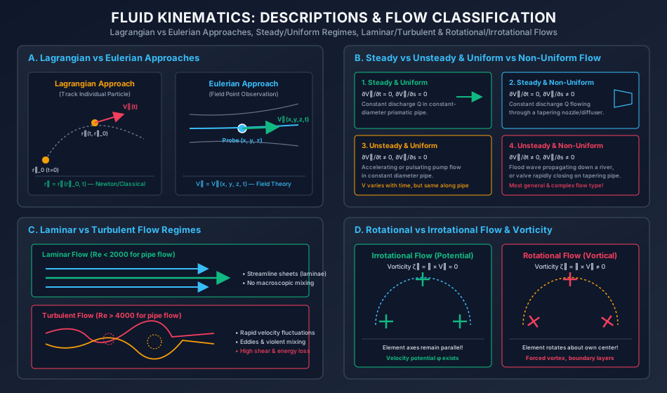
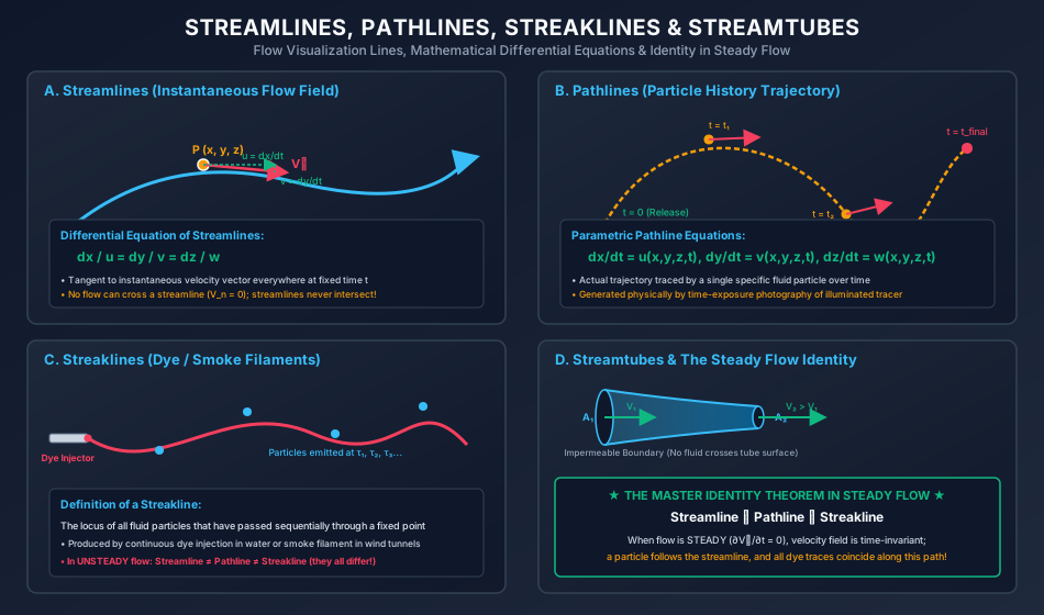
Diagram 2: Streamlines, Pathlines, Streaklines & Streamtubes
The following diagram details the geometry and differential equations of streamlines, pathlines, continuous dye streaklines, streamtube flux invariance, and the Master Identity Theorem in steady flow:
8. Worked Numerical Problems
Problem 1: Streamline and Pathline in a 2D Steady Flow Field (GATE Standard)
Statement: A steady two-dimensional velocity field is given by:
Where and are in meters.
- Determine the general differential equation of the streamlines and find the equation of the streamline passing through the point .
- Determine the parametric equations of the pathline of a fluid particle that was located at at time . Show that the Cartesian equation of the pathline is identical to the streamline.
- Calculate the magnitude of the velocity and acceleration of this particle at time .
Solution:
Part 1: Streamline Equation:
- Velocity components:
- Differential equation of streamline:
- Integrating both sides: (A family of rectangular hyperbolas!)
- For the streamline passing through :
Part 2: Pathline Equations:
-
Parametric rate of displacement:
At
At
-
Eliminating time by multiplying and :
The pathline equation is , which is completely identical to the streamline equation. (This verifies the theorem that in steady flow, streamlines and pathlines coincide).
Part 3: Kinematics at :
- Position of particle at : (Check: )
- Velocity components at :
- Velocity magnitude:
- Acceleration components (steady flow ):
- At :
- Total acceleration magnitude:
Problem 2: Divergence of Streamlines and Pathlines in Unsteady Flow (ESE Standard)
Statement: An unsteady two-dimensional velocity field is defined by:
Where are in meters and is in seconds.
- Determine the equation of the streamline passing through at the instantaneous time .
- Determine the parametric and Cartesian equations of the pathline of a fluid particle that passes through at time .
- Evaluate the position of the particle on the pathline at and compare it with the streamline passing through the same initial point, quantitatively proving their divergence.
Solution:
Part 1: Streamline at Passing Through :
- At the frozen instant :
- Streamline equation:
- Integrating:
- Passing through :
- Streamline at : (A straight line with slope )
Part 2: Pathline for Particle Released at at :
- For the -coordinate: At
- For the -coordinate: This is a first-order linear ordinary differential equation. Integrating factor: . Multiplying through by : Integrating by parts: Applying initial condition at :
- Eliminating using and :
Part 3: Quantitative Comparison at :
- Position of particle on pathline at :
- Let us evaluate where the streamline passing through at is at this -location ():
- Divergence: The actual physical particle is at , whereas the streamline passing through at that instant predicts . This rigorously proves that in unsteady flow, streamlines and pathlines completely diverge.
Problem 3: Parabolic Streakline in Unsteady Shear Flow (GATE / ESE Standard)
Statement: In a wind tunnel study, an unsteady velocity field is represented by:
Where is a constant horizontal speed and is a constant vertical acceleration parameter. Smoke is continuously injected from a fixed nozzle located at the origin starting at .
- Derive the equation of the instantaneous streamline passing through the origin at time .
- Derive the equation of the streakline observed at time .
- Show that the streakline is a parabola, and compare its slope at the origin with the instantaneous streamline.
Solution:
Part 1: Instantaneous Streamline at :
- At :
- Differential equation of streamline:
- Integrating for the streamline passing through the origin : (The instantaneous streamline is a straight line through the origin with slope )
Part 2: Streakline at : Consider an arbitrary smoke particle that was injected at the origin at emission time (where ).
-
Particle trajectory equations for :
-
At current observation time :
Expanding the squared bracket:
-
Substituting numerical values ():
Part 3: Comparison and Geometric Analysis:
- The Streakline is a Parabola: is a parabola opening downwards with vertex at:
- Slope at the Origin (): The slope of the streakline at the injection point is identical to the slope of the instantaneous streamline ().
- Curvature Divergence: Away from the origin, the streamline remains a straight line (, curvature ), whereas the streakline curves downward (). This demonstrates that while a streakline is tangent to the streamline at the injection point, it curves away in unsteady flow.
9. Common Traps, Fallacies & Edge Cases
Trap 1: Conflating Streamlines and Pathlines in Unsteady Flows
- The Fallacy: Assuming that because water flows along streamlines, an individual water particle must follow a streamline in any flow.
- The Physical Reality: A streamline is an instantaneous snapshot at time . In unsteady flow, the streamline orientation shifts continuously at every subsequent millisecond. The particle's pathline integrates the changing velocity vectors over time, completely diverging from the instantaneous streamline. Only in steady flow do they coincide.
Trap 2: Confusing Uniform Flow with Constant Flow Velocity
- The Fallacy: Assuming that "steady flow" and "uniform flow" mean the same thing.
- The Physical Reality:
- Steady: Independence from time ().
- Uniform: Independence from space along streamline (). A steady flow can be violently non-uniform (e.g., flow through a converging nozzle where velocity accelerates from to across space, but remains constant at every point in time).
Trap 3: Assuming Smoke or Dye in Wind Tunnels Traces Streamlines
- The Fallacy: Treating smoke plumes in wind tunnel aerodynamic tests as streamlines under gusty or oscillating wind conditions.
- The Physical Reality: Continuous smoke injection generates a streakline. If the flow has vortex shedding or unsteady gusting, the streakline diverges from the streamline. Only in steady wind tunnel flow does a smoke line accurately portray a streamline.
Trap 4: Thinking Zero Velocity Gradient Across Streamlines Means Uniform Flow
- The Fallacy: Assuming implies uniform flow.
- The Physical Reality: Uniformity requires velocity to remain constant along the streamline (). Variation perpendicular to the streamline () determines vorticity and shear stress, not spatial uniformity along the flow direction.
10. Multi-Exam Multi-Choice & Conventional Practice Set
Q1. GATE CE (1 Mark) — Steady Flow Line Equivalence
Question: Under which of the following conditions do streamlines, pathlines, and streaklines coincide identically?
- (A) Laminar flow
- (B) Irrotational flow
- (C) Steady flow
- (D) Uniform flow
Solution: In steady flow, the Eulerian velocity vector at every point in space is invariant in time (). A fluid particle follows the streamline, and all dye particles emitted sequentially from that point trace the exact same trajectory. Hence, streamlines, pathlines, and streaklines coincide identically in steady flow. Correct Answer: (C)
Q2. UPSC ESE (Paper-II) — Flow Classification of Sluice Gate Flow
Question: Water discharges from a reservoir under a constant head through a sluice gate into an open channel with expanding width. The flow is classified as:
- (A) Steady and uniform
- (B) Steady and non-uniform
- (C) Unsteady and uniform
- (D) Unsteady and non-uniform
Solution: Because the reservoir head is constant, flow properties at any point do not vary with time (). Because the channel width expands, flow velocity decreases along the flow path (). Hence, the flow is steady and non-uniform. Correct Answer: (B)
Q3. SSC JE — Streamline Differential Equation
Question: The differential equation of a streamline in a two-dimensional Cartesian velocity field is:
- (A)
- (B)
- (C)
- (D)
Solution: Along a streamline, the slope is tangent to the velocity vector: . Correct Answer: (B)
Q4. State AE — Definition of a Streamtube
Question: Which of the following statements is TRUE regarding a streamtube?
- (A) Fluid continuously enters through the walls of the streamtube.
- (B) Streamlines inside a streamtube can cross each other.
- (C) No fluid can cross the boundary surface of a streamtube.
- (D) The velocity at all points inside a streamtube must be uniform.
Solution: Because the boundary of a streamtube is formed entirely of streamlines, and the normal velocity across any streamline is zero (), no fluid can cross the surface of a streamtube. Correct Answer: (C)
Q5. RRB JE — Lagrangian vs Eulerian Approach
Question: The method of describing fluid motion by observing the velocity and pressure at fixed points in space as fluid passes by is known as:
- (A) Lagrangian method
- (B) Eulerian method
- (C) Control mass method
- (D) Particle trajectory method
Solution: The Eulerian framework defines velocity as a spatial field observed at fixed coordinates in space. Correct Answer: (B)
11. Cross-Subject Synthesis & Practical Field Applications
1. Structural Wind Engineering: Aeroelastic Bluff Body Testing
In the design of supertall skyscrapers (such as Burj Khalifa) and long-span cable-stayed bridges, wind tunnel testing employs smoke streaklines to identify aerodynamic separation points, wake vortex shedding, and stagnation lines. In steady flow tunnels, these streaklines reveal streamline curvature that dictates peak negative suction pressures on curtain wall cladding.
2. Environmental Engineering: Riverine Pollutant Plumes
When an industrial effluent or thermal discharge enters a river, continuous chemical tracer injection forms a physical streakline. Under steady river discharge, the streakline traces the streamline path, allowing environmental engineers to position downstream water intake wells outside the toxic concentration plume.
3. Open Channel Hydraulics: Transitions & Flumes
In the hydraulic design of Venturi flumes and canal transitions (IS 1192), converging streamline patterns produce convective acceleration, converting potential head into kinetic energy. Designers ensure smooth streamline curvature to prevent boundary layer separation and energy-dissipating eddy formation.
12. Comprehensive Summary & Formula Cheatsheet
Quick Revision Cards
================================================================================
                    FLUID KINEMATICS: FLOW LINES CHEATSHEET
================================================================================

1. DESCRIPTIONS OF FLUID MOTION:
   - Lagrangian: Track individual particle r⃗ = r⃗(t, r⃗_0)   [Classic Mechanics]
   - Eulerian:   Fixed field observation V⃗ = V⃗(x, y, z, t)  [Standard Fluid Flow]
   - Material Derivative: D/Dt = ∂/∂t + (V⃗ · ∇)

2. FLOW CLASSIFICATION (4-QUADRANT MATRIX):
   - Steady Flow:    ∂V⃗/∂t = 0  (Time-invariant)
   - Unsteady Flow:  ∂V⃗/∂t ≠ 0  (Changes with time)
   - Uniform Flow:   ∂V⃗/∂s = 0  (Constant along streamline at fixed instant)
   - Non-Uniform:    ∂V⃗/∂s ≠ 0  (Varies along streamline)
   - Laminar/Turbulent: Re = ρ V D / μ  (Pipe: Re < 2000 laminar, > 4000 turbulent)
   - Incompressible:   Ma = V / c < 0.30  (Δρ/ρ < 5%)
   - Irrotational:     Vorticity ζ⃗ = ∇ × V⃗ = 0  (Velocity potential φ exists)

3. FLOW LINES & TUBES:
   - Streamline: Tangent to velocity vector at instant t:
                 dx / u = dy / v = dz / w
                 * Cannot intersect, V_n = 0, no flow across streamline
   - Pathline:   Actual trajectory traced by particle over time:
                 dx/dt = u,  dy/dt = v,  dz/dt = w
   - Streakline: Locus of all particles passing through a fixed injection point
   - Streamtube: Bundle of streamlines; impermeable boundary (Q = const)

4. THE MASTER IDENTITY THEOREM:
   - In STEADY FLOW: Streamline ≡ Pathline ≡ Streakline  (Coincide identically!)
   - In UNSTEADY FLOW: Streamline ≠ Pathline ≠ Streakline (They all diverge!)
================================================================================
References & Standard Codes
- White, F. M., Fluid Mechanics, 8th Edition, McGraw-Hill Education, 2016.
- Streeter, V. L., Wylie, E. B., and Bedford, K. W., Fluid Mechanics, 9th Edition, McGraw-Hill, New York.
- Modi, P. N., and Seth, S. M., Hydraulics and Fluid Mechanics Including Hydraulics Machines, Standard Book House, New Delhi.
- Kundu, P. K., Cohen, I. M., and Dowling, D. R., Fluid Mechanics, 6th Edition, Academic Press.
- IS 1192:1981, Velocity-Area Methods for Measurement of Flow of Water in Open Channels, Bureau of Indian Standards.