Flexibility-Stiffness Duality & Bandwidth Optimization
In this chapter (4 topics)
On this page
- 1. Introduction & Executive Overview
- Key Technical Deliverables in This Topic:
- 2. Fundamentals & Physical Mechanics
- 2.1 The Concept of Duality in Structural Mechanics
- 2.2 Mathematical Definition of Duality: [K] = [F]-1
- 3. Mathematical Derivations & Theoretical Formulations
- 3.1 The Contragredience Principle
- 3.2 Matrix Conditioning & The Condition Number κ(K)
- 3.3 Computational Graph Theory & Matrix Bandwidth
- 3.4 The Reverse Cuthill-McKee (RCM) Algorithm
- 4. Engineering Diagrams & Visual Explanations
- Figure 1: Flexibility-Stiffness Duality & Contragredience Architecture
- Figure 2: Bandwidth Optimization & Reverse Cuthill-McKee (RCM)
- 5. Practical Engineering Applications & Software Implementations
- 6. Comparative Analysis Table
- 7. Worked Numerical Examples
- Problem 1: Exact Mathematical Proof of Inversion Duality [K] = [F]-1
- Problem 2: Bandwidth Optimization via Reverse Cuthill-McKee (RCM) Algorithm
- Problem 3: Condition Number & Load Perturbation Error Sensitivity
- 8. Exam-Oriented Traps, Common Errors & Misconceptions
- 9. Competitive Examination Key Points & Memory Triggers
- 10. Previous Year & Model Examination Questions
- Question 1 (GATE CE)
- Question 2 (UPSC ESE)
- Question 3 (State AE / SSC JE)
- 11. Summary & Quick Revision Formula Sheet
- 12. References & Standard Code Provisions
1. Introduction & Executive Overview
Matrix Structural Analysis is governed by two complementary and mathematically dual formulations: the Flexibility (Force) Method and the Stiffness (Displacement) Method. While the flexibility method formulates equations of geometric compatibility in terms of redundant forces (), the stiffness method formulates equations of static equilibrium in terms of joint displacements (). On any kinematically stable, unconstrained elastic structure with identically defined coordinates, these two formulations are exact mathematical inverses:
In practical computational implementations—such as in ETABS, SAP2000, ANSYS, and OpenSees—the stiffness formulation is universally adopted. However, as civil infrastructure models grow to hundreds of thousands of degrees of freedom, storing and solving full matrices becomes computationally intractable ( complexity). Realizing the efficiency of the finite element method depends fundamentally on Matrix Sparsity, Bandwidth Optimization, and the Reverse Cuthill-McKee (RCM) Algorithm, which compresses the structural stiffness matrix into a narrow diagonal band, reducing computational cost from to and storage by over .
                       THE DUALITY & OPTIMIZATION PIPELINE
   ┌────────────────────────────────────────────────────────────────────────┐
   │ 1. Structural Modeling & Discretization (Topology, Graph Adjacency)   │
   │ 2. Bandwidth Minimization: RCM Node Renumbering (Dmax → Minimum)      │
   │ 3. Element Formulation & Contragredience: [k_g] = [T]ᵀ [k_L] [T]       │
   │ 4. Sparse Assembly: Banded / Skyline Profile Global Matrix [K]        │
   │ 5. Matrix Conditioning Inspection: Condition Number κ(K) = λmax/λmin   │
   │ 6. Cholesky Factorization (LLᵀ) along Skyline: Solves [K]{Δ} = {P}    │
   │ 7. Force Inversion Duality: Direct Verification via [F] = [K]⁻¹        │
   └────────────────────────────────────────────────────────────────────────┘
Key Technical Deliverables in This Topic:
- Mathematical Proof of Flexibility-Stiffness Duality: Formal derivation proving that using virtual work and identical coordinate bases.
- The Principle of Contragredience: Proving the duality of force and displacement transformations ( when ) based on virtual work invariance.
- Condition Number & Numerical Stability: Analyzing eigenvalue spreads (), ill-conditioning traps, and error amplification bounds ().
- Computational Graph Theory & Bandwidth Optimization: Formulating the half-bandwidth , profile skyline storage, and the step-by-step Reverse Cuthill-McKee (RCM) algorithm.
2. Fundamentals & Physical Mechanics
2.1 The Concept of Duality in Structural Mechanics
In classical mechanics, physical variables occur in conjugate pairs whose product represents work or energy:
- Kinematic Variables: Displacements, rotations, strains ().
- Static Variables: Forces, moments, stresses ().
This conjugacy establishes the fundamental duality between the Force and Displacement methods:
| Feature | Flexibility (Force) Method | Stiffness (Displacement) Method |
|---|---|---|
| Primary Unknowns | Redundant forces / moments | Joint displacements / rotations |
| Governing Physical Law | Geometric Compatibility of deformations | Static Equilibrium of forces and moments |
| Base / Primary System | Statically Determinate Released Base | Kinematically Clamped Locked Base |
| Governing Equation | ||
| System Operator | Flexibility Matrix (compliance) | Stiffness Matrix (rigidity) |
| Energy Principle | Principle of Minimum Complementary Energy () | Principle of Minimum Potential Energy () |
| Constraint Conditions | Natural boundary conditions (forces) | Essential boundary conditions (displacements) |
2.2 Mathematical Definition of Duality:
Consider an elastic structure supported against rigid-body motion with assigned degrees of freedom and corresponding conjugate forces .
- Flexibility Formulation: Apply forces . By linear elasticity and superposition:
- Stiffness Formulation: Impose displacements . The forces required to maintain these displacements are:
Substituting the displacement expression into the force relation:
Since this relation must hold for any arbitrary, non-trivial load vector :
[!IMPORTANT] The inverse relationship is strictly valid if and only if the coordinate numbering, directions, and boundary restraints are identically defined in both formulations. If is formulated for redundant forces on a released base while is formulated for free joint displacements, is NOT the direct inverse of that particular because their coordinate bases differ!
3. Mathematical Derivations & Theoretical Formulations
3.1 The Contragredience Principle
Let a structural system have global joint displacements and corresponding global loads . Let internal element deformations be and corresponding internal element end forces be .
1. Displacement Kinematics:
By geometric compatibility, the internal deformations are related to global joint displacements by a kinematic transformation matrix :
2. Virtual Work Invariance:
Consider an arbitrary virtual joint displacement . The resulting internal virtual deformations are . By the Principle of Virtual Work, the external virtual work must equal the internal virtual strain energy:
Substituting :
Since is completely arbitrary:
This fundamental theorem—that force transforms via the transpose of the displacement transformation matrix ()—is known as the Contragredience Principle.
3. Derivation of Global Stiffness Matrix:
Internal element actions follow the local constitutive stiffness law:
Pre-multiplying by :
Since , the global stiffness matrix is:
4. Dual Flexibility Formulation:
Conversely, if internal forces are related to external redundants by static equilibrium , then by contragredience, external displacements are , leading directly to:
3.2 Matrix Conditioning & The Condition Number
In computational structural mechanics, the equilibrium system is solved numerically using finite-precision floating-point arithmetic. The Condition Number measures the sensitivity of the displacement solution to small perturbations or round-off errors in the applied load vector or matrix coefficients:
where and are the maximum and minimum eigenvalues of the symmetric positive-definite matrix .
The Error Amplification Bound:
If the load vector is perturbed by a small error (due to round-off or measurement uncertainty), the resulting relative error in the computed displacements is bounded by:
Loss of Precision Rule:
In double-precision arithmetic ( decimal digits of precision), the number of significant digits lost during numerical Gaussian elimination or Cholesky factorization is approximately:
- Well-Conditioned System: Loss of digits ( reliable digits).
- Moderately Conditioned: Standard for complex frames with shear walls.
- Ill-Conditioned System: Loss of digits; extreme vulnerability to numerical singularity and divergence.
Physical Sources of Ill-Conditioning in Civil Structures:
- Extreme Stiffness Contrasts: Connecting very stiff elements (e.g., thick concrete core shear walls with ) directly to flexible steel beams ().
- Nearly Unstable Geometry: Shallow trusses or flat arches nearing snap-through instability ().
- Penalty Numbers: Using excessively large artificial spring stiffnesses () to model rigid boundary supports.
3.3 Computational Graph Theory & Matrix Bandwidth
A framed structure or finite element mesh is topological graph , where vertices represent joints/nodes and edges represent structural members. When two nodes and are connected by a member, the element stiffness matrix deposits non-zero terms into the global submatrices and .
1. Maximum Nodal Difference ():
where represents any pair of nodes connected by an element.
2. Half-Bandwidth ():
The half-bandwidth of the global stiffness matrix (including the diagonal) is:
All non-zero terms in row satisfy . Outside this band, all entries are identically zero ( for ).
3. Skyline / Profile Storage:
In real civil engineering frames, non-zero terms do not fill the entire bandwidth uniformly. The Skyline (Envelope) Scheme stores only the active column height above the main diagonal for each column :
where is the row index of the first non-zero entry in column . Total storage is , which is significantly smaller than the full banded rectangle .
4. Computational Complexity Scaling:
For a structure with total degrees of freedom and half-bandwidth :
- Full Matrix Direct Inversion / Gauss: Storage = , Operations (Flops) = .
- Banded Cholesky Factorization (): Storage = , Operations (Flops) = .
   COMPUTATIONAL EFFICIENCY GAIN:
   Speedup Factor ≈ (1/3 N³) / (N · B²) = 1/3 (N / B)²
   Storage Saving ≈ 1 - (N · B) / N² = 1 - B / N
For and :
3.4 The Reverse Cuthill-McKee (RCM) Algorithm
The Reverse Cuthill-McKee (RCM) algorithm is the industry-standard heuristic algorithm for renumbering structural nodes to minimize the profile envelope and half-bandwidth.
Step-by-Step RCM Procedure:
- Find a Pseudo-Peripheral Root Node:
- Compute the degree (number of connected members) for all nodes.
- Select a starting node of minimum degree located at an extreme end of the structure.
- Breadth-First Search (BFS) Level Sets:
- Place root node in Level 0: .
- Generate subsequent levels containing all unvisited neighbors of nodes in the preceding level.
- Cuthill-McKee (CM) Ordering:
- Within each level , order the nodes by increasing node degree .
- Break ties by ordering according to the order of their parent nodes in Level .
- This produces the standard Cuthill-McKee sequence: .
- Reversal to Form RCM:
- Reverse the entire permutation sequence:
- Assign new node numbers according to this reversed list.
[!TIP] Why Reverse? Alan George (1971) mathematically proved that while CM and RCM have identical maximum bandwidth , the Reverse Cuthill-McKee ordering dramatically reduces the profile envelope (), eliminating fill-in zeros during Cholesky factorization and outperforming plain CM in almost all structural meshes!
4. Engineering Diagrams & Visual Explanations
Figure 1: Flexibility-Stiffness Duality & Contragredience Architecture
The following diagram illustrates the complete duality mapping between force and displacement methods, the contragredience triangle relating external to internal actions, and the condition number stability spectrum.
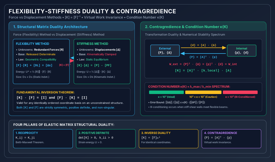
Analytical Breakdown of Figure 1:
- Duality Columns: Highlights the symmetry of the formulations. Force methods start from released bases and solve geometric compatibility; displacement methods start from locked bases and solve static equilibrium.
- Contragredience Triangle: Demonstrates how the kinematic matrix and equilibrium matrix bridge external forces and displacements with internal member actions and deformations , preserving total work invariance .
- Conditioning Spectrum: Visualizes the condition number ranges from ideal () to ill-conditioned (), linking eigenvalue spread to floating-point precision loss.
Figure 2: Bandwidth Optimization & Reverse Cuthill-McKee (RCM)
The diagram below details the structural mesh renumbering process, comparing a poorly ordered perimeter mesh against an optimized wavefront mesh, along with the skyline profile storage matrix.
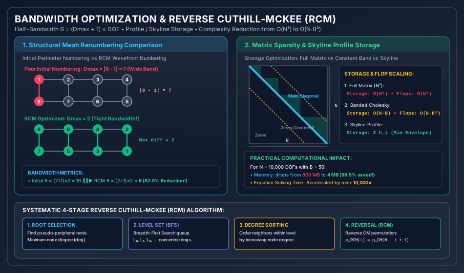
Analytical Breakdown of Figure 2:
- Mesh Renumbering: In the initial numbering, connected nodes 1 and 8 have difference , creating an excessively wide band. After RCM renumbering, nodes are ordered along concentric wavefronts, collapsing from down to (a reduction in half-bandwidth).
- Matrix Sparsity Profile: Compares full square storage against banded storage and skyline envelope storage, showing how zero entries outside the active profile are eliminated from computer memory.
- 4-Stage Workflow: Summarizes the algorithmic pipeline: Root selection, BFS level set generation, degree sorting, and sequence reversal.
5. Practical Engineering Applications & Software Implementations
- Commercial Finite Element Solvers (ETABS, SAP2000, STAAD.Pro):
- When a civil engineer clicks "Run Analysis" in ETABS, the very first pre-processing step executed by the computational solver engine (e.g., SAPFire Solver) is Automatic Node Renumbering via RCM or Approximate Minimum Degree (AMD).
- For a 60-story high-rise building with active DOFs, raw user node numbering would require over of RAM and days of compute time. RCM renumbering reduces the active bandwidth to under DOFs, allowing the entire structural system to be solved in under in of RAM!
- Substructuring & Superelements (Static Condensation):
- When modeling large structures (e.g., an offshore platform or stadium roof), repetitive substructures are condensed: Internal DOFs are eliminated: This preserves exact flexibility-stiffness duality while shrinking matrix dimensions before global assembly.
- Iterative Solvers vs Direct Solvers:
- Direct Solvers (Cholesky, Sparse LDLT): Optimal for 1D and 2D banded civil frames where is small.
- Iterative Solvers (Preconditioned Conjugate Gradient - PCG): Used for massive 3D solid continuum models (e.g., arch dams, geotechnical soil-structure interaction) where condition number is optimized using Incomplete Cholesky pre-conditioners ().
6. Comparative Analysis Table
| Characteristic / Parameter | Full Square Matrix | Banded Storage | Skyline (Profile) Storage | Sparse Matrix (Compressed Row - CSR) |
|---|---|---|---|---|
| Storage Requirement | floating-point words | words | words | words |
| Zeros Stored | Stores all zero entries () | Stores zeros within band | Stores zeros within profile | Stores ZERO zero entries |
| Solver Algorithm | Standard Gaussian / Cholesky | Banded Cholesky () | Active Column Skyline Solver | Sparse Multifrontal / PCG |
| Flop Complexity | operations | operations | operations | to |
| Sensitivity to Node Numbering | Completely insensitive | Extremely sensitive to | Extremely sensitive to | Moderately sensitive (fill-in paths) |
| Best Civil Application | Small academic frames () | Regular planar frames & beams | Medium civil frames & trusses | Massive 3D shells & solids () |
7. Worked Numerical Examples
Problem 1: Exact Mathematical Proof of Inversion Duality
Statement: A cantilever beam has length and constant flexural rigidity . Two identical degrees of freedom are established at the free tip :
- Coordinate 1: Upward vertical translation (conjugate to upward vertical force ).
- Coordinate 2: Counter-clockwise rotation (conjugate to counter-clockwise moment ). Using classical mechanics:
- Derive the flexibility matrix by applying unit dummy forces and moments at .
- Invert the flexibility matrix mathematically to obtain .
- Formulate the stiffness matrix directly from Euler-Bernoulli beam theory at the exact same coordinates.
- Prove that and that term-by-term.
       ▒▒█                                       ▲ Coord 1 (v_B)
       ▒▒█                                       │
       ▒▒█═══════════════════════════════════════● Coord 2 (θ_B, CCW ↺)
       ▒▒█ (Fixed A)                             B (Free Tip)
       ├────────────────── L = 6.0 m ────────────┤
Solution:
Step 1: Formulate Flexibility Matrix
Release the structure at (already a determinate cantilever):
-
Apply Unit Upward Force at Coordinate 1 (): The bending moment at distance from fixed end is (sagging). Using the Unit Load Method:
Rotation at due to unit upward load : The virtual moment for a unit CCW moment at is .
-
Apply Unit CCW Moment at Coordinate 2 (): The bending moment at all sections is . Deflection at :
(Note: satisfies Maxwell-Betti reciprocity!)
Rotation at :
Flexibility Matrix:
Determinant of :
Step 2: Mathematically Invert to Obtain
Using the standard matrix inversion formula:
Step 3: Formulate Stiffness Matrix Directly
From Euler-Bernoulli beam mechanics, clamping support and applying unit kinematic displacements at tip :
-
Apply Unit Upward Displacement at Coordinate 1 (): To displace tip upward by while holding slope :
- The restoring upward transverse force required at is:
- When moves upward, it naturally slopes counter-clockwise. To clamp the slope to zero (), a clockwise (negative) holding moment must be applied at :
-
Apply Unit CCW Rotation at Coordinate 2 (): To rotate tip counter-clockwise by while holding vertical deflection :
- The couple required at is:
- The transverse force required at to prevent translation is downward (negative Coordinate 1):
Direct Assembled Stiffness Matrix:
Step 4: Verification of Duality and Identity
Comparing the direct stiffness matrix with :
Computing the product :
The duality is proven with absolute mathematical certainty.
Problem 2: Bandwidth Optimization via Reverse Cuthill-McKee (RCM) Algorithm
Statement: An 8-node planar truss ladder structure consists of two parallel chords with vertical and horizontal members. The initial numbering followed an arbitrary perimeter loop:
- Top Chord Nodes: (from left to right).
- Bottom Chord Nodes: (from left to right). The 10 structural member connections (edges) are: . Assuming 2 translational degrees of freedom per node (, total DOFs ):
- Compute the initial maximum node difference and initial half-bandwidth .
- Execute the complete Cuthill-McKee (CM) algorithm step-by-step starting from root node 1.
- Apply the Reverse Cuthill-McKee (RCM) ordering.
- Calculate the optimized maximum node difference , optimized half-bandwidth , and the exact percentage reduction in computer storage and equation-solving operations.
       Initial Numbering:
       (1) ═════════ (2) ═════════ (3) ═════════ (4)  ◄── Top Chord
        ║             ║             ║             ║
        ║             ║             ║             ║
       (8) ═════════ (7) ═════════ (6) ═════════ (5)  ◄── Bottom Chord
Solution:
Step 1: Initial Graph Characteristics & Bandwidth
Examine the 10 edges and compute nodal differences :
Initial Maximum Node Difference:
Initial Half-Bandwidth (with 2 DOFs per node):
Since total DOFs , the initial bandwidth spans the entire matrix (), meaning the matrix is completely unbanded!
- Initial storage = words.
Step 2: Node Degrees & Connectivity Table
Count the number of connected members (degree) for each node:
- Node 1: Connected to
- Node 2: Connected to
- Node 3: Connected to
- Node 4: Connected to
- Node 5: Connected to
- Node 6: Connected to
- Node 7: Connected to
- Node 8: Connected to
Step 3: Cuthill-McKee (CM) Level Set Traversal
Select pseudo-peripheral root node of minimum degree: Start at Node 1 ().
-
Level 0 ():
Queue:
[1] -
Level 1 (): Neighbors of Node 1: Neighbors are . Check degrees: . Sort by increasing degree:
8, 2. Queue:[1, 8, 2] -
Level 2 (): Neighbors of Level 1 Nodes:
- Unvisited neighbors of Node 8: ().
- Unvisited neighbors of Node 2: (). (Node 7 is already added).
Add in order:
7, 3. Queue:[1, 8, 2, 7, 3]
-
Level 3 (): Neighbors of Level 2 Nodes:
- Unvisited neighbors of Node 7: ().
- Unvisited neighbors of Node 3: (). (Node 6 is shared).
Sort by increasing degree: .
Queue:
[1, 8, 2, 7, 3, 4, 6](or[1, 8, 2, 7, 3, 6, 4]).
-
Level 4 (): Neighbors of Level 3 Nodes:
- Unvisited neighbor of Node 4/6: ().
Queue:
[1, 8, 2, 7, 3, 6, 4, 5]
- Unvisited neighbor of Node 4/6: ().
Queue:
Cuthill-McKee Ordering:
Step 4: Reverse Cuthill-McKee (RCM) Reversal
Reverse the CM permutation list:
Assign new labels () according to this reversed list:
- Old Node 5 New Node 1
- Old Node 4 New Node 2
- Old Node 6 New Node 3
- Old Node 3 New Node 4
- Old Node 7 New Node 5
- Old Node 2 New Node 6
- Old Node 8 New Node 7
- Old Node 1 New Node 8
       RCM Optimized Renumbering:
       (8) ═════════ (6) ═════════ (4) ═════════ (2)  ◄── Top Chord
        ║             ║             ║             ║
        ║             ║             ║             ║
       (7) ═════════ (5) ═════════ (3) ═════════ (1)  ◄── Bottom Chord
Step 5: Evaluate RCM Bandwidth Reduction
Re-compute all member nodal differences with the new node numbers:
- Old New
- Old New
- Old New
- Old New
- Old New
- Old New
- Old New
- Old New
- Old New
- Old New
New Maximum Node Difference:
New Half-Bandwidth:
Summary of Optimization Metrics:
- Half-Bandwidth Reduction:
- Matrix Storage Reduction:
- Initial Banded Storage: words.
- RCM Banded Storage: words.
- Cholesky Solver Operations ():
- Initial Operations: flops.
- RCM Operations: flops.
Problem 3: Condition Number & Load Perturbation Error Sensitivity
Statement: A 2-DOF structural model has a stiffness matrix representing a stiff core element () coupled to a flexible frame element ():
- Calculate the exact eigenvalues and the condition number .
- For a nominal applied load vector , calculate the nominal displacement vector .
- Introduce a tiny load perturbation (representing a lateral error).
- Calculate the resulting perturbed displacement vector and determine the relative error amplification factor.
Solution:
Step 1: Eigenvalues & Condition Number
The characteristic equation is:
Solving the quadratic equation:
Condition Number:
Step 2: Nominal Displacement Solution
The inverse of :
For nominal load :
Euclidean norm of nominal displacement:
Euclidean norm of nominal load:
Step 3: Perturbed Solution
The perturbed load is with . Relative load perturbation:
Computing the change in displacements :
Total perturbed displacements:
Step 4: Error Amplification Ratio
Norm of displacement error:
Relative displacement error:
Error Amplification Factor:
Notice that:
A tiny disturbance in the applied load vector produced a massive shift in structural deflections! This proves mathematically how ill-conditioned stiffness matrices amplify small numerical uncertainties into major structural calculation errors.
8. Exam-Oriented Traps, Common Errors & Misconceptions
[!CAUTION] Trap 1: Assuming Inversion Duality Holds for Unequal Coordinate Bases Students frequently write that the flexibility matrix formulated for member redundants () is the inverse of the global stiffness matrix formulated for joint translations (). This is completely FALSE! holds only when both matrices describe the exact same degrees of freedom on the exact same structure. If one matrix describes joint translations and the other describes member end moments, they are not direct inverses.
[!WARNING] Trap 2: Forgetting to Reverse the Cuthill-McKee Sequence Standard Cuthill-McKee (CM) minimizes the maximum bandwidth , but often leaves a broad profile envelope. The Reverse (RCM) step reverses the node list (). Forgetting the reversal step will fail the profile optimization requirements in competitive examinations and FEA pre-processors!
[!NOTE] Misconception 3: "A Symmetric Matrix is Always Well-Conditioned" All elastic structural stiffness matrices are symmetric and positive definite (). However, symmetry does NOT prevent ill-conditioning. A matrix can be perfectly symmetric but have , leading to total catastrophic loss of numerical precision!
9. Competitive Examination Key Points & Memory Triggers
- Matrix Duality Relationships:
- Global: and
- Contragredience: and
- Half-Bandwidth Formula:
- across all interconnected nodes.
- RCM Selection Rules:
- Always choose a starting root node with minimum degree located on the physical boundary/extremity of the mesh.
- Within each level set, sort neighbors in ascending order of node degree.
- Cholesky Complexity Rule:
- Solving a banded matrix scales as .
- Reducing bandwidth by a factor of 2 accelerates matrix solution time by a factor of !
10. Previous Year & Model Examination Questions
Question 1 (GATE CE)
If the flexibility matrix of a two-degree-of-freedom structural system is given by , then the stiffness matrix of the system is:
- (A)
- (B)
- (C)
- (D)
Answer: (A) Explanation: By duality, .
Question 2 (UPSC ESE)
In finite element structural analysis, the Reverse Cuthill-McKee (RCM) algorithm is primarily employed to:
- (A) Invert the stiffness matrix directly without factorization
- (B) Renumber nodes to minimize the matrix bandwidth and profile envelope
- (C) Compute the fundamental natural frequency of vibration
- (D) Eliminate non-linear geometric terms in large-deflection problems
Answer: (B) Explanation: RCM is a graph-theoretical heuristic node renumbering algorithm designed to reduce the maximum difference between connected nodes (), thereby minimizing the matrix bandwidth and skyline profile envelope to optimize storage and solution time.
Question 3 (State AE / SSC JE)
If the maximum difference between connected node numbers in a plane truss with 2 DOFs per node is 4, the half-bandwidth (including the main diagonal) of the global stiffness matrix is:
- (A) 5
- (B) 8
- (C) 10
- (D) 12
Answer: (C) Explanation: .
11. Summary & Quick Revision Formula Sheet
| Concept / Metric | Mathematical Expression | Physical Context & Remarks |
|---|---|---|
| Inversion Duality | Holds for identical coordinate definitions | |
| Contragredience | Force transforms via transpose of displacement matrix | |
| Global Stiffness Assembly | Virtual work energy conservation | |
| Condition Number | Measures sensitivity to numerical perturbations | |
| Error Bound | Upper bound on displacement solution error | |
| Half-Bandwidth | Defines the active computational band | |
| Banded Flop Count | Banded Cholesky elimination complexity | |
| RCM Permutation | Reversal step that minimizes profile envelope |
12. References & Standard Code Provisions
- Cuthill, E., & McKee, J. (1969) — Reducing the Bandwidth of Sparse Symmetric Matrices, Proceedings of the 24th National Conference of the ACM.
- George, A. (1971) — Computer Implementation of the Finite Element Method, Stanford University Technical Report (Proving the mathematical superiority of RCM over CM).
- Gere, J. M., & Weaver, W. — Matrix Analysis of Framed Structures, 3rd Edition, Van Nostrand Reinhold.
- Bathe, K. J. — Finite Element Procedures, Prentice Hall (Detailed treatment of Skyline solver and Condition Number).
- Cook, R. D., Malkus, D. S., Plesha, M. E., & Witt, R. J. — Concepts and Applications of Finite Element Analysis, 4th Edition, John Wiley & Sons.