SA-02-02 Chapter 02 · Energy Methods

Castigliano's Theorems, Betti's Law & Maxwell's Reciprocal Theorem

In this chapter (3 topics)
On this page
  1. 1. Executive Summary & Historical Context
  2. 2. Fundamental Energy Formulations: U vs U*
  3. 2.1 Strain Energy (U) and Complementary Strain Energy (U*)
  4. 2.2 The Energy Conservation Duality Law
  5. 3. Castigliano's First Theorem (Stiffness Formulation)
  6. 3.1 Theorem Statement
  7. 3.2 Proof via Virtual Displacements
  8. 4. Castigliano's Second Theorem (Flexibility Formulation)
  9. 4.1 Theorem Statement
  10. 4.2 Leibniz Differentiation Under the Integral Sign
  11. 4.3 The Mathematical Identity between Castigliano II and the Unit Load Method
  12. 4.4 The Dummy / Fictitious Load Technique (Q0 → 0)
  13. 5. Betti's Reciprocal Work Theorem (1872)
  14. 5.1 Theorem Statement
  15. 5.2 Mathematical Proof based on Strain Energy Path-Independence
  16. 6. Maxwell's Reciprocal Deflection Theorem (1864)
  17. 6.1 Theorem Statement
  18. 6.2 Structural Symmetry of Flexibility and Stiffness Matrices
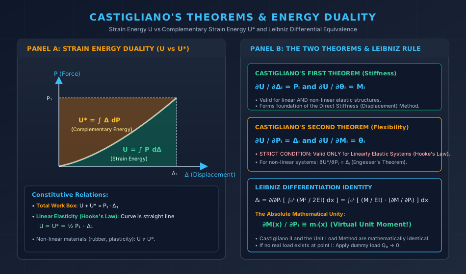
  19. 6.3 Cross-Reciprocity: Linear Force vs Applied Moment
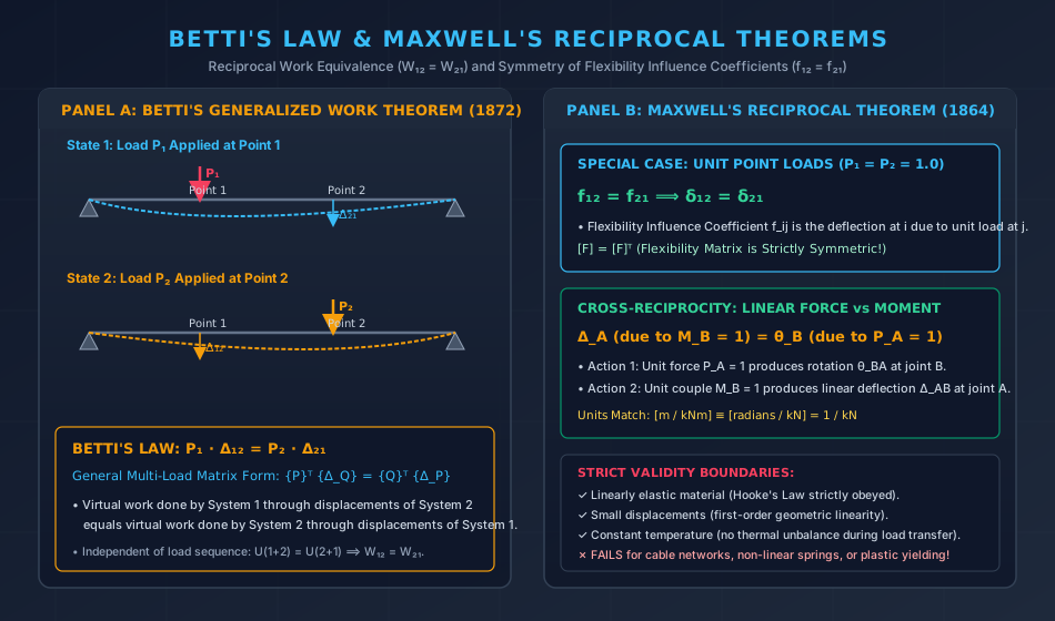
  20. 6.4 Four Mandatory Conditions for Reciprocity:
  21. 7. Engineering Visualizations
  22. 7.1 Castigliano's Theorems & Constitutive Energy Duality
  23. 7.2 Betti's Law & Maxwell's Reciprocal Theorems
  24. 8. Comparative Analysis Matrix
  25. 9. Solved Numerical Examples with Rigorous Verification
  26. Example 1: Quarter-Circular Cantilever Curved Beam under Tip Load
  27. Example 2: Rigorous Verification of Maxwell's Reciprocal Theorem on an Overhanging Beam
  28. Example 3: Betti's Reciprocal Law with Force-Moment Cross-Reciprocity
  29. 10. Common Pitfalls, Exam Traps & Misconceptions
  30. 10.1 Applying Castigliano's Second Theorem to Non-Linear Materials
  31. 10.2 Differentiating After Integrating (The Algebraic Explosion)
  32. 10.3 Forgetting to Zero the Fictitious Dummy Load
  33. 10.4 Units Trap in Cross-Reciprocity
  34. 11. Competitive Examination Practice & Master Formula Sheet
  35. 11.1 Representative Competitive Exam Questions
  36. 11.2 Master Formula Sheet

1. Executive Summary & Historical Context

Energy methods represent the most mathematically rigorous and unifying approach to structural mechanics. In the 1860s and 1870s, three European engineers and mathematicians established the bedrock theorems that govern elastic structural analysis:

  1. James Clerk Maxwell (1864): Discovered the reciprocal deflection relationship for elastic structures (fij=fjif_{ij} = f_{ji}), proving that flexibility matrices are strictly symmetric.
  2. Enrico Betti (1872): Generalized Maxwell's work into the theorem of reciprocal work for arbitrary multi-force systems (∑PiΔi′=∑Pi′Δi\sum P_i \Delta_i' = \sum P_i' \Delta_i).
  3. Carlo Alberto Castigliano (1873, published 1879): Formulated the two fundamental energy differentiation theorems in his masterwork Théorie de l'équilibre des systèmes élastiques, revolutionizing the analysis of statically indeterminate bridges and roof trusses.

Together with the Unit Load Method, Castigliano's Theorems and Reciprocal Laws form the direct bridge between classical manual force analysis and modern computerized finite element formulations.


2. Fundamental Energy Formulations: UU vs U∗U^*

2.1 Strain Energy (UU) and Complementary Strain Energy (U∗U^*)

Consider a general elastic body subjected to generalized forces P1,P2,…,PnP_1, P_2, \dots, P_n producing corresponding generalized displacements Δ1,Δ2,…,Δn\Delta_1, \Delta_2, \dots, \Delta_n:

Force P ^
        |         /
     P₁ +--------*
        |       /|
        |  U*  / |
        |     /  |  U
        |    /   |
      0 +---*----+-----> Displacement Δ
            0   Δ₁
  1. Strain Energy (UU): The work done by internal stresses during deformation, expressed as a function of displacements:

    U(Δ1,Δ2,…,Δn)=∫V(∫0ϵσ:dϵ)dVU(\Delta_1, \Delta_2, \dots, \Delta_n) = \int_V \left( \int_0^\epsilon \mathbf{\sigma} : d\mathbf{\epsilon} \right) dV

    Geometrically, UU is the area under the load-displacement curve (U=∫P dΔU = \int P \, d\Delta).

  2. Complementary Strain Energy (U∗U^*): The dual energy potential, expressed as a function of forces:

    U∗(P1,P2,…,Pn)=∫V(∫0σϵ:dσ)dVU^*(P_1, P_2, \dots, P_n) = \int_V \left( \int_0^\sigma \mathbf{\epsilon} : d\mathbf{\sigma} \right) dV

    Geometrically, U∗U^* is the area above the load-displacement curve (U∗=∫Δ dPU^* = \int \Delta \, dP).

2.2 The Energy Conservation Duality Law

The sum of strain energy and complementary strain energy equals the total rectangular bounding work box:

U+U∗=∑i=1nPiΔi\boxed{U + U^* = \sum_{i=1}^n P_i \Delta_i}

Linear vs Non-Linear Elasticity:

  • Linearly Elastic Material (Hooke's Law): The load-displacement curve is a straight line (P=KΔP = K \Delta). The diagonal splits the bounding rectangle into two equal triangles: U=U∗=12∑i=1nPiΔi=12∫0LM2EI dx+12∑j=1mPj2LjAjEj\boxed{U = U^* = \frac{1}{2} \sum_{i=1}^n P_i \Delta_i = \frac{1}{2} \int_0^L \frac{M^2}{EI} \, dx + \frac{1}{2} \sum_{j=1}^m \frac{P_j^2 L_j}{A_j E_j}}
  • Non-Linearly Elastic Material: If P∝ΔnP \propto \Delta^n (n≠1n \ne 1), the curve is non-linear. Therefore, U≠U∗U \ne U^*, and ordinary energy formulas must strictly distinguish between UU and U∗U^*.

3. Castigliano's First Theorem (Stiffness Formulation)

3.1 Theorem Statement

Castigliano's First Theorem: For any elastic structure (whether linearly or non-linearly elastic) supported in a manner that prevents rigid-body motion and kept at constant temperature, the first partial derivative of the total strain energy UU with respect to any particular displacement Δi\Delta_i equals the generalized force PiP_i acting at that point in the direction of Δi\Delta_i:

∂U∂Δi=Piand∂U∂θi=Mi\boxed{\frac{\partial U}{\partial \Delta_i} = P_i \quad \text{and} \quad \frac{\partial U}{\partial \theta_i} = M_i}

3.2 Proof via Virtual Displacements

Let the structure undergo an infinitesimal virtual variation in displacement δΔi\delta\Delta_i while all other displacements are held fixed:

  • Change in external work: δWext=Pi⋅δΔi\delta W_{\text{ext}} = P_i \cdot \delta\Delta_i
  • Change in internal strain energy: δU=∂U∂Δi⋅δΔi\delta U = \frac{\partial U}{\partial \Delta_i} \cdot \delta\Delta_i By conservation of energy (δWext=δU\delta W_{\text{ext}} = \delta U):
Pi⋅δΔi=∂U∂Δi⋅δΔi  ⟹  Pi=∂U∂ΔiP_i \cdot \delta\Delta_i = \frac{\partial U}{\partial \Delta_i} \cdot \delta\Delta_i \implies P_i = \frac{\partial U}{\partial \Delta_i}

Engineering Implication: Castigliano's First Theorem forms the foundation of the Displacement / Direct Stiffness Method and Finite Element Formulations, because it expresses forces in terms of known or unknown nodal displacements:

{P}=[K]{Δ}whereKij=∂2U∂Δi∂Δj\{P\} = [K] \{\Delta\} \quad \text{where} \quad K_{ij} = \frac{\partial^2 U}{\partial \Delta_i \partial \Delta_j}

4. Castigliano's Second Theorem (Flexibility Formulation)

4.1 Theorem Statement

Castigliano's Second Theorem: In any linearly elastic structure at constant temperature with unyielding supports, the first partial derivative of the total strain energy UU with respect to any external applied force PiP_i equals the displacement Δi\Delta_i of the point of application of that force along its line of action:

∂U∂Pi=Δiand∂U∂Mi=θi\boxed{\frac{\partial U}{\partial P_i} = \Delta_i \quad \text{and} \quad \frac{\partial U}{\partial M_i} = \theta_i}

For non-linearly elastic materials, this theorem is valid only when expressed in terms of Complementary Strain Energy U∗U^* (known historically as Engesser's Theorem, 1889):

∂U∗∂Pi=Δi\frac{\partial U^*}{\partial P_i} = \Delta_i

4.2 Leibniz Differentiation Under the Integral Sign

Evaluating total strain energy U=∫0LM22EIdxU = \int_0^L \frac{M^2}{2EI} dx and then differentiating with respect to PiP_i can become unwieldy. By applying Leibniz's rule for differentiation under the integral sign:

Δi=∂∂Pi[∫0LM(x)22EI dx]=∫0L2M(x)2EI(∂M(x)∂Pi)dx\Delta_i = \frac{\partial}{\partial P_i} \left[ \int_0^L \frac{M(x)^2}{2EI} \, dx \right] = \int_0^L \frac{2 M(x)}{2EI} \left( \frac{\partial M(x)}{\partial P_i} \right) dx Δi=∫0LM(x)EI(∂M(x)∂Pi)dx\boxed{\Delta_i = \int_0^L \frac{M(x)}{EI} \left( \frac{\partial M(x)}{\partial P_i} \right) dx}

Similarly, for a pin-jointed truss:

Δi=∑j=1mPjLjAjEj(∂Pj∂Pi)\boxed{\Delta_i = \sum_{j=1}^m \frac{P_j L_j}{A_j E_j} \left( \frac{\partial P_j}{\partial P_i} \right)}

4.3 The Mathematical Identity between Castigliano II and the Unit Load Method

Notice the physical meaning of the term ∂M(x)∂Pi\frac{\partial M(x)}{\partial P_i}:

  • If M(x)M(x) is a linear function of applied load PiP_i, the derivative ∂M(x)∂Pi\frac{\partial M(x)}{\partial P_i} represents the bending moment produced when PiP_i increases by unity (1.01.0).
  • This is identically equal to the virtual unit moment mi(x)m_i(x) in the Dummy Unit Load Method:
∂M(x)∂Pi≡mi(x)and∂Pj∂Pi≡kj\boxed{\frac{\partial M(x)}{\partial P_i} \equiv m_i(x) \quad \text{and} \quad \frac{\partial P_j}{\partial P_i} \equiv k_j}

Thus, Castigliano's Second Theorem and the Unit Load Method are mathematically identical for linearly elastic systems!

4.4 The Dummy / Fictitious Load Technique (Q0→0Q_0 \to 0)

If a deflection or rotation is required at a point or in a direction where no real load exists:

  1. Apply an imaginary fictitious load Q0Q_0 (or moment M0M_0) at that point in the desired direction.
  2. Formulate the bending moment M(x,Q0)M(x, Q_0) including Q0Q_0.
  3. Differentiate before integration: ∂M(x,Q0)∂Q0\frac{\partial M(x, Q_0)}{\partial Q_0}.
  4. Set Q0=0Q_0 = 0 inside the integrand prior to performing the integration:
Δ=∫0LM(x,Q0)EI(∂M(x,Q0)∂Q0)dx∣Q0=0\boxed{\Delta = \left. \int_0^L \frac{M(x, Q_0)}{EI} \left( \frac{\partial M(x, Q_0)}{\partial Q_0} \right) dx \right|_{Q_0 = 0}}

This eliminates messy algebraic terms and avoids squaring large expressions.


5. Betti's Reciprocal Work Theorem (1872)

5.1 Theorem Statement

Betti's Law (Generalized Reciprocal Work Theorem): In any linearly elastic structure at constant temperature with unyielding supports, if two independent, separate equilibrium systems of forces {P}\{P\} and {Q}\{Q\} act upon the structure, the virtual work done by the forces of System {P}\{P\} acting through the displacements produced by System {Q}\{Q\} equals the virtual work done by the forces of System {Q}\{Q\} acting through the displacements produced by System {P}\{P\}:

∑i=1nPi⋅ΔQ,i=∑j=1mQj⋅ΔP,j\boxed{\sum_{i=1}^n P_i \cdot \Delta_{Q,i} = \sum_{j=1}^m Q_j \cdot \Delta_{P,j}}

In matrix notation:

{P}T{ΔQ}={Q}T{ΔP}\boxed{\{P\}^T \{\Delta_Q\} = \{Q\}^T \{\Delta_P\}}
System 1 (P-System):           System 2 (Q-System):
    ↓ P₁                           ↓ Q₁
====▲=============▲====        ====▲=============▲====
    ↓ Δ_{P,1}     ↓ Δ_{P,2}        ↓ Δ_{Q,1}     ↓ Δ_{Q,2}

5.2 Mathematical Proof based on Strain Energy Path-Independence

Because an elastic structure is conservative, the total strain energy stored when both Systems {P}\{P\} and {Q}\{Q\} are applied must be independent of the order of loading.

  • Sequence 1: Apply System {P}\{P\} first, then System {Q}\{Q\}:

    1. System {P}\{P\} applied from 00 to {P}\{P\}: U1=12{P}T{ΔP}U_1 = \frac{1}{2} \{P\}^T \{\Delta_P\}
    2. System {Q}\{Q\} applied while System {P}\{P\} remains at full magnitude:
      • Work done by {Q}\{Q\} on its own deformations: 12{Q}T{ΔQ}\frac{1}{2} \{Q\}^T \{\Delta_Q\}
      • Work done by constant forces {P}\{P\} riding through new displacements {ΔQ}\{\Delta_Q\}: {P}T{ΔQ}\{P\}^T \{\Delta_Q\}
    Utotal, 1=12{P}T{ΔP}+12{Q}T{ΔQ}+{P}T{ΔQ}U_{\text{total, 1}} = \frac{1}{2} \{P\}^T \{\Delta_P\} + \frac{1}{2} \{Q\}^T \{\Delta_Q\} + \{P\}^T \{\Delta_Q\}
  • Sequence 2: Apply System {Q}\{Q\} first, then System {P}\{P\}:

    Utotal, 2=12{Q}T{ΔQ}+12{P}T{ΔP}+{Q}T{ΔP}U_{\text{total, 2}} = \frac{1}{2} \{Q\}^T \{\Delta_Q\} + \frac{1}{2} \{P\}^T \{\Delta_P\} + \{Q\}^T \{\Delta_P\}

Equating Utotal, 1=Utotal, 2U_{\text{total, 1}} = U_{\text{total, 2}}:

{P}T{ΔQ}={Q}T{ΔP}■\{P\}^T \{\Delta_Q\} = \{Q\}^T \{\Delta_P\} \quad \blacksquare

6. Maxwell's Reciprocal Deflection Theorem (1864)

6.1 Theorem Statement

Maxwell's Reciprocal Theorem is the single-degree-of-freedom corollary of Betti's Law, published 8 years earlier:

Maxwell's Reciprocal Theorem: In any linearly elastic structure, the deflection at point 1 due to a unit load at point 2 is equal in magnitude to the deflection at point 2 due to a unit load at point 1:

f12=f21orδ12=δ21\boxed{f_{12} = f_{21} \quad \text{or} \quad \delta_{12} = \delta_{21}}

Where fijf_{ij} is the flexibility influence coefficient (displacement at coordinate ii caused by a unit force at coordinate jj).

6.2 Structural Symmetry of Flexibility and Stiffness Matrices

A direct mathematical consequence of Maxwell's Theorem is that:

  1. The Flexibility Matrix [F][F] of any linear elastic structure is strictly symmetric: [F]=[F]T  ⟺  fij=fji[F] = [F]^T \iff f_{ij} = f_{ji}
  2. Because the stiffness matrix is the inverse of flexibility ([K]=[F]−1[K] = [F]^{-1}), the Stiffness Matrix [K][K] is also strictly symmetric: [K]=[K]T  ⟺  Kij=Kji[K] = [K]^T \iff K_{ij} = K_{ji}

6.3 Cross-Reciprocity: Linear Force vs Applied Moment

Maxwell's reciprocity applies across dissimilar generalized coordinates (forces and couples):

  • Let Action 1 be a unit concentrated force PA=1P_A = 1 at joint AA.
  • Let Action 2 be a unit concentrated moment MB=1M_B = 1 at joint BB.

By Betti's Law (PA⋅ΔA2=MB⋅θB1P_A \cdot \Delta_{A2} = M_B \cdot \theta_{B1}):

(1.0 kN)⋅ΔAB=(1.0 kNm)⋅θBA(1.0\text{ kN}) \cdot \Delta_{AB} = (1.0\text{ kNm}) \cdot \theta_{BA} ΔAB=θBA\boxed{\Delta_{AB} = \theta_{BA}}

Units Consistency:

  • ΔAB\Delta_{AB}: Linear deflection at AA due to unit moment at BB   ⟹  [mkNm]=[1kN]\implies \left[\frac{\text{m}}{\text{kNm}}\right] = \left[\frac{1}{\text{kN}}\right]
  • θBA\theta_{BA}: Angular rotation (radians) at BB due to unit force at AA   ⟹  [radkN]=[1kN]\implies \left[\frac{\text{rad}}{\text{kN}}\right] = \left[\frac{1}{\text{kN}}\right] Both quantities have identical dimensions of [F]−1[F]^{-1}!

6.4 Four Mandatory Conditions for Reciprocity:

Maxwell's and Betti's theorems are valid if and only if:

  1. Material is strictly linearly elastic (Hooke's Law holds; no plastic yielding).
  2. Deformations are small (first-order geometric linearity; no PP-Δ\Delta or cable sag effects).
  3. Temperature is constant during the load process (no thermal strains).
  4. Supports are rigid and unyielding (no support settlements).

7. Engineering Visualizations

7.1 Castigliano's Theorems & Constitutive Energy Duality

Castigliano's Theorems & Energy Duality

7.2 Betti's Law & Maxwell's Reciprocal Theorems

Betti's Law & Maxwell's Reciprocal Theorems

8. Comparative Analysis Matrix

Feature Castigliano's 1st Theorem Castigliano's 2nd Theorem Betti's Reciprocal Law Maxwell's Reciprocal Theorem
Differentiating Variable Displacement (Δi\Delta_i or θi\theta_i) Force (PiP_i or MiM_i) No differentiation (Integral work) No differentiation (Direct coefficients)
Resulting Quantity Conjugate Force (PiP_i or MiM_i) Conjugate Displacement (Δi\Delta_i or θi\theta_i) Work equivalence (W12=W21W_{12} = W_{21}) Cross-displacement equality (fij=fjif_{ij} = f_{ji})
Material Elasticity Linear AND Non-linear elastic Linearly elastic ONLY (unless U∗U^* used) Linearly elastic ONLY Linearly elastic ONLY
Primary Structural Role Formulates Stiffness Matrix [K][K] Solves deflections & redundants Proves matrix symmetry; ILD Muller-Breslau Validates flexibility coefficients [F][F]
Dummy Load Needed? No (applied at kinematic DOFs) Yes (if no real load exists at point) No No

9. Solved Numerical Examples with Rigorous Verification

Example 1: Quarter-Circular Cantilever Curved Beam under Tip Load

Problem Statement:

A uniform curved circular cantilever beam ABAB of radius R=1.5 mR = 1.5\text{ m} lies in a vertical plane. It is rigidly fixed at base AA (θ=0\theta = 0) and free at tip BB (θ=π/2\theta = \pi/2). The cross-section has flexural rigidity EI=5000 kNm2EI = 5000\text{ kNm}^2. A concentrated vertical downward load P=10 kNP = 10\text{ kN} is applied at free tip BB.

Using Castigliano's Second Theorem, calculate:

  1. The vertical deflection Δv\Delta_v at free end BB.
  2. The horizontal deflection Δh\Delta_h at free end BB (using a fictitious dummy load).
       B (Free)  ↓ P = 10 kN
      /
     /  Quadrant of Radius R = 1.5 m
    /
   |
   |
===A=== Fixed base

Solution:

Step 1: Coordinate System and Geometry: Let θ\theta be measured from horizontal base AA to any section (0≤θ≤π/20 \le \theta \le \pi/2).

  • Coordinates of section: x(θ)=Rsin⁡θx(\theta) = R \sin\theta, y(θ)=R(1−cos⁡θ)y(\theta) = R(1 - \cos\theta).
  • Coordinates of tip BB: xB=Rx_B = R, yB=Ry_B = R.
  • Differential arc length: ds=R dθds = R \, d\theta.

Step 2: Real Bending Moment M(θ)M(\theta): Horizontal lever arm from section to line of action of vertical load PP at BB:

Armx=xB−x(θ)=R−Rsin⁡θ=R(1−sin⁡θ)\text{Arm}_x = x_B - x(\theta) = R - R\sin\theta = R(1 - \sin\theta) M(θ)=PR(1−sin⁡θ)M(\theta) = P R (1 - \sin\theta)

Step 3: Vertical Deflection Δv\Delta_v at Tip BB:

∂M(θ)∂P=R(1−sin⁡θ)\frac{\partial M(\theta)}{\partial P} = R (1 - \sin\theta) Δv=∫0π/2M(θ)EI(∂M∂P)ds=PR3EI∫0π/2(1−sin⁡θ)2dθ\Delta_v = \int_0^{\pi/2} \frac{M(\theta)}{EI} \left( \frac{\partial M}{\partial P} \right) ds = \frac{P R^3}{EI} \int_0^{\pi/2} (1 - \sin\theta)^2 d\theta

Expanding (1−sin⁡θ)2=1−2sin⁡θ+sin⁡2θ(1 - \sin\theta)^2 = 1 - 2\sin\theta + \sin^2\theta:

  1. ∫0π/21 dθ=π2\int_0^{\pi/2} 1 \, d\theta = \frac{\pi}{2}
  2. ∫0π/2−2sin⁡θ dθ=−2[−cos⁡θ]0π/2=−2(0−(−1))=−2\int_0^{\pi/2} -2\sin\theta \, d\theta = -2 [-\cos\theta]_0^{\pi/2} = -2(0 - (-1)) = -2
  3. ∫0π/2sin⁡2θ dθ=π4\int_0^{\pi/2} \sin^2\theta \, d\theta = \frac{\pi}{4}

Total integral:

Iv=π2−2+π4=3π4−2≈2.356194−2=0.356194I_v = \frac{\pi}{2} - 2 + \frac{\pi}{4} = \frac{3\pi}{4} - 2 \approx 2.356194 - 2 = 0.356194 Δv=0.356194⋅PR3EI\Delta_v = 0.356194 \cdot \frac{P R^3}{EI}

Substituting P=10 kNP = 10\text{ kN}, R=1.5 mR = 1.5\text{ m}, EI=5000 kNm2EI = 5000\text{ kNm}^2:

Δv=0.356194×10×1.535000=0.356194×33.755000=2.4043×10⁻³ m=2.404 mm↓\Delta_v = 0.356194 \times \frac{10 \times 1.5^3}{5000} = 0.356194 \times \frac{33.75}{5000} = 2.4043 \times 10^{-3}\text{ m} = \mathbf{2.404\text{ mm} \downarrow}

Step 4: Horizontal Deflection Δh\Delta_h at Tip BB (Fictitious Load Q0Q_0): Apply an imaginary rightward horizontal force Q0Q_0 at tip BB. Vertical lever arm from section to Q0Q_0:

Army=yB−y(θ)=R−R(1−cos⁡θ)=Rcos⁡θ\text{Arm}_y = y_B - y(\theta) = R - R(1 - \cos\theta) = R\cos\theta M(θ,Q0)=PR(1−sin⁡θ)+Q0Rcos⁡θM(\theta, Q_0) = P R (1 - \sin\theta) + Q_0 R \cos\theta ∂M(θ,Q0)∂Q0=Rcos⁡θ\frac{\partial M(\theta, Q_0)}{\partial Q_0} = R\cos\theta

Evaluate derivative at Q0=0Q_0 = 0:

Δh=∫0π/2PR(1−sin⁡θ)EI(Rcos⁡θ)R dθ=PR3EI∫0π/2(cos⁡θ−sin⁡θcos⁡θ)dθ\Delta_h = \int_0^{\pi/2} \frac{P R(1 - \sin\theta)}{EI} (R\cos\theta) R \, d\theta = \frac{P R^3}{EI} \int_0^{\pi/2} (\cos\theta - \sin\theta\cos\theta) d\theta

Integrating:

  1. ∫0π/2cos⁡θ dθ=[sin⁡θ]0π/2=1−0=1\int_0^{\pi/2} \cos\theta \, d\theta = [\sin\theta]_0^{\pi/2} = 1 - 0 = 1
  2. ∫0π/2sin⁡θcos⁡θ dθ=[sin⁡2θ2]0π/2=12−0=12\int_0^{\pi/2} \sin\theta\cos\theta \, d\theta = \left[ \frac{\sin^2\theta}{2} \right]_0^{\pi/2} = \frac{1}{2} - 0 = \frac{1}{2}

Total integral:

Ih=1−12=0.5000I_h = 1 - \frac{1}{2} = 0.5000 Δh=0.5000⋅PR3EI=0.5000×10×1.535000=3.3750×10⁻³ m=3.375 mm→\Delta_h = 0.5000 \cdot \frac{P R^3}{EI} = 0.5000 \times \frac{10 \times 1.5^3}{5000} = 3.3750 \times 10^{-3}\text{ m} = \mathbf{3.375\text{ mm} \to}

Example 2: Rigorous Verification of Maxwell's Reciprocal Theorem on an Overhanging Beam

Problem Statement:

A beam ABCABC has total length 8.0 m8.0\text{ m}. It is simply supported at AA (x=0x = 0) and BB (x=6.0 mx = 6.0\text{ m}), with an overhanging span BCBC of length a=2.0 ma = 2.0\text{ m} ending at tip CC (x=8.0 mx = 8.0\text{ m}). Point DD is located at the exact midspan of ABAB (x=3.0 mx = 3.0\text{ m}). The flexural rigidity is constant EIEI.

  1. Compute the downward deflection at midspan DD due to a unit downward load at overhang tip CC (δDC\delta_{DC}).
  2. Compute the downward deflection at overhang tip CC due to a unit downward load at midspan DD (δCD\delta_{CD}).
  3. Verify that δDC=δCD\delta_{DC} = \delta_{CD}.
A (Pin)              D (Midspan)             B (Roller)         C (Tip)
▲------------------------|-----------------------▲-----------------|
0                       3.0 m                   6.0 m             8.0 m
|================== Span L = 6.0 m ==============|=== Overhang 2.0 m ==|

Solution:

Step 1: Case 1 — Deflection at DD due to Unit Load at CC (δDC\delta_{DC}): Apply real downward load PC=1.0P_C = 1.0 at CC (x=8.0 mx = 8.0\text{ m}).

  • Support Reactions: ∑MA=0  ⟹  RB×6.0−1.0×8.0=0  ⟹  RB=86=43↑\sum M_A = 0 \implies R_B \times 6.0 - 1.0 \times 8.0 = 0 \implies R_B = \frac{8}{6} = \frac{4}{3} \uparrow ∑Fy=0  ⟹  RA+43−1.0=0  ⟹  RA=−13↓(Downward)\sum F_y = 0 \implies R_A + \frac{4}{3} - 1.0 = 0 \implies R_A = -\frac{1}{3} \downarrow \quad (\text{Downward})
  • Real Bending Moment Function MC(x)M_C(x) in main span ABAB (0≤x≤6.0 m0 \le x \le 6.0\text{ m}): MC(x)=RA⋅x=−13x(Hogging throughout)M_C(x) = R_A \cdot x = -\frac{1}{3} x \quad (\text{Hogging throughout})

To find deflection at DD (x=3.0 mx = 3.0\text{ m}), apply a dummy unit downward load at DD:

  • Virtual Reactions: rA=0.5r_A = 0.5, rB=0.5r_B = 0.5.
  • Virtual Bending Moment Function mD(x)m_D(x):
    • Segment ADAD (0≤x≤3.0 m0 \le x \le 3.0\text{ m}): mD(x)=0.5xm_D(x) = 0.5 x
    • Segment DBDB (3.0≤x≤6.0 m3.0 \le x \le 6.0\text{ m}): mD(x)=0.5(6.0−x)m_D(x) = 0.5(6.0 - x)
    • Overhang BCBC (6.0≤x≤8.0 m6.0 \le x \le 8.0\text{ m}): mD(x)=0m_D(x) = 0

Now compute δDC\delta_{DC}:

δDC=∫06MC(x)mD(x)EI dx=∫03(−x3)(x2)EI dx+∫36(−x3)(6−x2)EI dx\delta_{DC} = \int_0^6 \frac{M_C(x) m_D(x)}{EI} \, dx = \int_0^3 \frac{(-\frac{x}{3})(\frac{x}{2})}{EI} \, dx + \int_3^6 \frac{(-\frac{x}{3})(\frac{6 - x}{2})}{EI} \, dx
  1. First integral (00 to 33): ∫03−x26 dx=[−x318]03=−2718=−1.5EI\int_0^3 -\frac{x^2}{6} \, dx = \left[ -\frac{x^3}{18} \right]_0^3 = -\frac{27}{18} = -\frac{1.5}{EI}
  2. Second integral (33 to 66): ∫36(−x+x26)dx=[−x22+x318]36\int_3^6 \left( -x + \frac{x^2}{6} \right) dx = \left[ -\frac{x^2}{2} + \frac{x^3}{18} \right]_3^6
    • At x=6x = 6: −362+21618=−18+12=−6-\frac{36}{2} + \frac{216}{18} = -18 + 12 = -6
    • At x=3x = 3: −92+2718=−4.5+1.5=−3-\frac{9}{2} + \frac{27}{18} = -4.5 + 1.5 = -3
    Difference=−6−(−3)=−3.0\text{Difference} = -6 - (-3) = -3.0
δDC=−1.5−3.0EI=−4.5EI(Negative indicates upward displacement at D)\delta_{DC} = \frac{-1.5 - 3.0}{EI} = \mathbf{-\frac{4.5}{EI}} \quad (\text{Negative indicates upward displacement at } D)

Step 2: Case 2 — Deflection at CC due to Unit Load at DD (δCD\delta_{CD}): Apply real downward load PD=1.0P_D = 1.0 at DD (x=3.0 mx = 3.0\text{ m}).

  • Support Reactions: RA=0.5R_A = 0.5, RB=0.5R_B = 0.5.
  • Real Moment MD(x)M_D(x):
    • Segment ADAD (0≤x≤30 \le x \le 3): MD(x)=0.5xM_D(x) = 0.5 x
    • Segment DBDB (3≤x≤63 \le x \le 6): MD(x)=0.5(6−x)M_D(x) = 0.5(6 - x)
    • Overhang BCBC (6≤x≤86 \le x \le 8): MD(x)=0M_D(x) = 0

To find deflection at CC, apply a dummy unit downward load at CC:

  • Virtual Moment mC(x)m_C(x) in span ABAB: mC(x)=−13xm_C(x) = -\frac{1}{3} x.

Now compute δCD\delta_{CD}:

δCD=∫06MD(x)mC(x)EI dx=∫03(x2)(−x3)EI dx+∫36(6−x2)(−x3)EI dx\delta_{CD} = \int_0^6 \frac{M_D(x) m_C(x)}{EI} \, dx = \int_0^3 \frac{(\frac{x}{2})(-\frac{x}{3})}{EI} \, dx + \int_3^6 \frac{(\frac{6 - x}{2})(-\frac{x}{3})}{EI} \, dx δCD=∫03−x26EI dx+∫36−x+x26EI dx=−1.5−3.0EI=−4.5EI\delta_{CD} = \int_0^3 -\frac{x^2}{6EI} \, dx + \int_3^6 \frac{-x + \frac{x^2}{6}}{EI} \, dx = \frac{-1.5 - 3.0}{EI} = \mathbf{-\frac{4.5}{EI}} δDC=δCD=−4.5EI■\boxed{\delta_{DC} = \delta_{CD} = -\frac{4.5}{EI}} \quad \blacksquare

Maxwell's Reciprocal Theorem is validated to full mathematical precision!


Example 3: Betti's Reciprocal Law with Force-Moment Cross-Reciprocity

Problem Statement:

A cantilever beam ABAB of span L=4.0 mL = 4.0\text{ m} is fixed at AA and free at BB, with flexural rigidity EI=20,000 kNm2EI = 20,000\text{ kNm}^2. Point CC is the midspan (x=2.0 mx = 2.0\text{ m}).

  • State 1: A concentrated vertical load P1=50 kNP_1 = 50\text{ kN} is applied at tip BB.
  • State 2: A concentrated clockwise couple M2=100 kNmM_2 = 100\text{ kNm} is applied at midspan CC.

Verify Betti's Reciprocal Law:

P1⋅ΔB2=M2⋅θC1P_1 \cdot \Delta_{B2} = M_2 \cdot \theta_{C1}

Solution:

Step 1: State 1 Analysis (Load P1=50 kNP_1 = 50\text{ kN} at BB):

  • Moment function: M1(x)=−P1(L−x)=−50(4−x)=−200+50xM_1(x) = -P_1(L - x) = -50(4 - x) = -200 + 50x (for 0≤x≤4 m0 \le x \le 4\text{ m}).
  • To find rotation θC1\theta_{C1} at midspan CC, apply a dummy unit couple mθ=1.0m_\theta = 1.0 at CC:
    • From x=0x = 0 to x=2 mx = 2\text{ m}: m(x)=1.0m(x) = 1.0
    • From x=2x = 2 to x=4 mx = 4\text{ m}: m(x)=0m(x) = 0
θC1=∫02(−200+50x)(1.0)EI dx=1EI[−200x+25x2]02=−400+100EI=−300EI radians\theta_{C1} = \int_0^2 \frac{(-200 + 50x)(1.0)}{EI} \, dx = \frac{1}{EI} \left[ -200x + 25x^2 \right]_0^2 = \frac{-400 + 100}{EI} = -\frac{300}{EI}\text{ radians} ∣θC1∣=300EI rad|\theta_{C1}| = \frac{300}{EI}\text{ rad}

Step 2: State 2 Analysis (Couple M2=100 kNmM_2 = 100\text{ kNm} at CC):

  • Moment function:
    • From x=0x = 0 to x=2 mx = 2\text{ m}: M2(x)=−M2=−100 kNmM_2(x) = -M_2 = -100\text{ kNm} (constant hogging)
    • From x=2x = 2 to x=4 mx = 4\text{ m}: M2(x)=0M_2(x) = 0
  • To find deflection ΔB2\Delta_{B2} at tip BB, apply a dummy downward unit load p=1.0p = 1.0 at BB:
    • mB(x)=−1.0(4−x)=−(4−x)m_B(x) = -1.0(4 - x) = -(4 - x)
ΔB2=∫02(−100)(−(4−x))EI dx=100EI∫02(4−x) dx=100EI[4x−x22]02\Delta_{B2} = \int_0^2 \frac{(-100)(-(4 - x))}{EI} \, dx = \frac{100}{EI} \int_0^2 (4 - x) \, dx = \frac{100}{EI} \left[ 4x - \frac{x^2}{2} \right]_0^2 ΔB2=100EI[8−2]=600EI m\Delta_{B2} = \frac{100}{EI} [8 - 2] = \frac{600}{EI}\text{ m}

Step 3: Verification of Betti's Reciprocal Equation:

LHS=P1⋅ΔB2=(50 kN)×(600EI m)=30,000EI kNm\text{LHS} = P_1 \cdot \Delta_{B2} = (50\text{ kN}) \times \left( \frac{600}{EI}\text{ m} \right) = \mathbf{\frac{30,000}{EI}\text{ kNm}} RHS=M2⋅θC1=(100 kNm)×(300EI rad)=30,000EI kNm\text{RHS} = M_2 \cdot \theta_{C1} = (100\text{ kNm}) \times \left( \frac{300}{EI}\text{ rad} \right) = \mathbf{\frac{30,000}{EI}\text{ kNm}} LHS≡RHS=30,000EI kNm■\boxed{\text{LHS} \equiv \text{RHS} = \frac{30,000}{EI}\text{ kNm}} \quad \blacksquare

Both virtual work quantities match identically, confirming cross-reciprocity between linear force and bending couple.


10. Common Pitfalls, Exam Traps & Misconceptions

10.1 Applying Castigliano's Second Theorem to Non-Linear Materials

  • Trap: Using ∂U∂P=Δ\frac{\partial U}{\partial P} = \Delta for non-linear elastic springs, cables, or concrete cracking.
  • Rule: Castigliano's 2nd Theorem requires U=U∗U = U^*. If the material is non-linear (P=cΔn,n≠1P = c \Delta^n, n \ne 1), you must use Engesser's Theorem: ∂U∗∂Pi=Δi(never ∂U∂Pi)\frac{\partial U^*}{\partial P_i} = \Delta_i \quad \left( \text{never } \frac{\partial U}{\partial P_i} \right)

10.2 Differentiating After Integrating (The Algebraic Explosion)

  • Trap: Integrating U=∫M22EIdxU = \int \frac{M^2}{2EI} dx first into a massive algebraic equation, and then differentiating with respect to PP.
  • Rule: Always apply Leibniz's rule and differentiate under the integral sign first: Δ=∫MEI(∂M∂P)dx\Delta = \int \frac{M}{EI} \left( \frac{\partial M}{\partial P} \right) dx This halves computational effort and allows zeroing dummy loads before integrating.

10.3 Forgetting to Zero the Fictitious Dummy Load

  • Trap: Leaving dummy load Q0Q_0 in the final equation.
  • Rule: The fictitious load Q0Q_0 has no physical reality. After computing ∂M∂Q0\frac{\partial M}{\partial Q_0}, set Q0=0Q_0 = 0 in the expression for M(x)M(x) immediately before carrying out the definite integration.

10.4 Units Trap in Cross-Reciprocity

  • Trap: Claiming that ΔAB=θBA\Delta_{AB} = \theta_{BA} is dimensionally impossible because deflection is in meters and rotation is in radians.
  • Clarification: Deflection per unit moment has units mkNm=1kN\frac{\text{m}}{\text{kNm}} = \frac{1}{\text{kN}}. Rotation per unit force has units radkN=1kN\frac{\text{rad}}{\text{kN}} = \frac{1}{\text{kN}} (radians are dimensionless). The units match identically.

11. Competitive Examination Practice & Master Formula Sheet

11.1 Representative Competitive Exam Questions

Question 1 (GATE CE):

Castigliano's First Theorem is applicable to:

  • (A) Linearly elastic structures only
  • (B) Non-linearly elastic structures only
  • (C) Both linearly and non-linearly elastic structures
  • (D) Statically determinate structures only

Answer: (C)
Explanation: Castigliano's First Theorem (∂U/∂Δi=Pi\partial U / \partial \Delta_i = P_i) depends only on conservation of energy and virtual displacements; it is valid for all elastic materials. Castigliano's Second Theorem (∂U/∂Pi=Δi\partial U / \partial P_i = \Delta_i) is the one restricted to linear elasticity.


Question 2 (UPSC ESE):

According to Maxwell's reciprocal theorem, the flexibility influence coefficient fijf_{ij} satisfies:

  • (A) fij=−fjif_{ij} = - f_{ji}
  • (B) fij=fjif_{ij} = f_{ji}
  • (C) fij⋅fji=1f_{ij} \cdot f_{ji} = 1
  • (D) fij+fji=0f_{ij} + f_{ji} = 0

Answer: (B)
Explanation: Maxwell's theorem proves fij=fjif_{ij} = f_{ji}, establishing the symmetry of structural flexibility matrices.


Question 3 (SSC JE):

The first derivative of strain energy with respect to a concentrated load gives:

  • (A) Slope at that point
  • (B) Deflection along the line of action of the load
  • (C) Shear force at that point
  • (D) Bending moment at that point

Answer: (B)
Explanation: By Castigliano's Second Theorem, ∂U∂P=Δ\frac{\partial U}{\partial P} = \Delta.


11.2 Master Formula Sheet

Law / TheoremMathematical FormulationScope & RestrictionsStrain Energy BoxU+U∗=∑PiΔiUniversal for all elastic systemsLinear Elastic EquivalenceU=U∗=12∑PiΔiHooke’s Law strictly validCastigliano’s 1st Theorem∂U∂Δi=Pi,∂U∂θi=MiLinear and Non-linear elasticityCastigliano’s 2nd Theorem∂U∂Pi=Δi,∂U∂Mi=θiLinearly elastic systems ONLYEngesser’s Theorem∂U∗∂Pi=ΔiNon-linearly elastic systemsLeibniz Integral IdentityΔi=∫0LMEI(∂M∂Pi)dx∂M∂Pi≡mi(x) (Unit Moment)Betti’s Reciprocal Law∑PiΔQ,i=∑QjΔP,j{P}T{ΔQ}={Q}T{ΔP}Maxwell’s Reciprocal Theoremfij=fji  ⟹  [F]=[F]TFlexibility matrix symmetryCross-ReciprocityΔAB(MB=1)=θBA(PA=1)Consistent units: [1/kN]\begin{array}{|l|l|l|} \hline \textbf{Law / Theorem} & \textbf{Mathematical Formulation} & \textbf{Scope \& Restrictions} \\ \hline \text{Strain Energy Box} & U + U^* = \sum P_i \Delta_i & \text{Universal for all elastic systems} \\ \hline \text{Linear Elastic Equivalence} & U = U^* = \frac{1}{2} \sum P_i \Delta_i & \text{Hooke's Law strictly valid} \\ \hline \text{Castigliano's 1st Theorem} & \frac{\partial U}{\partial \Delta_i} = P_i, \quad \frac{\partial U}{\partial \theta_i} = M_i & \text{Linear and Non-linear elasticity} \\ \hline \text{Castigliano's 2nd Theorem} & \frac{\partial U}{\partial P_i} = \Delta_i, \quad \frac{\partial U}{\partial M_i} = \theta_i & \text{Linearly elastic systems ONLY} \\ \hline \text{Engesser's Theorem} & \frac{\partial U^*}{\partial P_i} = \Delta_i & \text{Non-linearly elastic systems} \\ \hline \text{Leibniz Integral Identity} & \Delta_i = \int_0^L \frac{M}{EI} \left( \frac{\partial M}{\partial P_i} \right) dx & \frac{\partial M}{\partial P_i} \equiv m_i(x) \text{ (Unit Moment)} \\ \hline \text{Betti's Reciprocal Law} & \sum P_i \Delta_{Q,i} = \sum Q_j \Delta_{P,j} & \{P\}^T \{\Delta_Q\} = \{Q\}^T \{\Delta_P\} \\ \hline \text{Maxwell's Reciprocal Theorem} & f_{ij} = f_{ji} \implies [F] = [F]^T & \text{Flexibility matrix symmetry} \\ \hline \text{Cross-Reciprocity} & \Delta_{AB} (M_B = 1) = \theta_{BA} (P_A = 1) & \text{Consistent units: } [1/\text{kN}] \\ \hline \end{array}