SA-03-02 Chapter 03 · Classical Indeterminate Structures

Clapeyron's Three-Moment Equation for Continuous Beams

Prerequisites
Static Indeterminacy of Beams, Trusses & Rigid Frames (2D & 3D) SA-01-01 , Kinematic Indeterminacy & Degrees of Freedom SA-01-02 , Moment-Area Theorems (Mohr's Theorems) & Conjugate Beam Method SOM-07-03 , Propped Cantilevers & Fixed Beams: Classical Indeterminate Formulations SA-03-01
Keywords
three-moment equation · clapeyron theorem · continuous beams · support moments · fictitious span · support sinking
In this chapter (4 topics)
On this page
  1. 1. Introduction & Engineering Significance
  2. 1.1 Structural Advantages of Continuous Beams
  3. 1.2 Degree of Static Indeterminacy
  4. 2. Mathematical Formulation & First-Principles Derivation
  5. 2.1 Geometric Compatibility at Intermediate Support B
  6. 2.2 Decomposition of Bending Moment Diagram
  7. 2.3 The Canonical Three-Moment Equation
  8. 2.4 Special Case: Homogeneous Material and Constant Cross-Section (EI = constant)
  9. 3. Standard Loading Terms (frac6 A barxL) Reference Table
  10. 4. Engineering Diagrams & Visual Explanations
  11. 4.1 Geometric Derivation & BMD Superposition
  12. 4.2 Special Boundary Conditions: Fictitious Span & Support Sinking
  13. 5. Treatment of Boundary Conditions
  14. 5.1 Simply Supported / Roller Free Ends
  15. 5.2 Cantilever Overhangs
  16. 5.3 Fixed Ends (The Fictitious Zero-Span Method)
  17. 6. Step-by-Step Analytical Procedure
  18. 7. Solved Numerical Examples
  19. Example 1: Two-Span Continuous Beam with Combined UDL and Central Point Load
  20. Example 2: Continuous Beam with Fixed End at Support A (Fictitious Span Application)
  21. Example 3: Effect of Support Settlement (Differential Sinking)
  22. 8. Practical Applications & Design Codes (IS 456 & IS 800)
  23. 8.1 Moment Redistribution in Reinforced Concrete (IS 456:2000 Clause 37.1)
  24. 8.2 Deflection Control in Continuous Beams (IS 456 Clause 23.2.1)
  25. 9. Comparative Matrix: Classical Methods of Indeterminate Beam Analysis
  26. 10. Common Misconceptions & Exam Traps
  27. 1. Centroid Measurement Inversion
  28. 2. The Fictitious Span Parameter Error
  29. 3. Intermediate Support Reaction Calculation
  30. 4. Sinking Sign Convention
  31. 11. Practice Problems
  32. Problem 1 (GATE CE Standard)
  33. Problem 2 (UPSC ESE Conventional Standard)
  34. 12. Quick Revision Formula Summary

1. Introduction & Engineering Significance

A continuous beam is a structural flexural member supported over three or more supports along its length. Unlike a series of disconnected simply supported beams, a continuous beam maintains rotational slope continuity (θ\theta) across its intermediate supports. This structural continuity induces negative (hogging) bending moments over the intermediate supports, which directly reduces the maximum positive (sagging) moments in the spans.

Simply Supported Series:
[▲]================[▲] [▲]================[▲]
     Span 1: Max Sagging = wL²/8             Span 2: Max Sagging = wL²/8
     Support Moment = 0                      Support Moment = 0

Continuous Beam:
[▲]================[▲]================[▲]
     Span 1: Max Sagging ≈ 0.070 wL²         Span 2: Max Sagging ≈ 0.070 wL²
     Intermediate Support Moment = -wL²/8 (Hogging relieves span sagging!)

1.1 Structural Advantages of Continuous Beams

  1. Substantial Reduction in Span Bending Moments: By mobilizing hogging resistance over piers and columns, peak sagging moments in adjacent spans are reduced by 30%30\% to 45%45\%. This allows shallower beam depths, saving concrete and structural steel.
  2. Enhanced Flexural Stiffness and Lower Deflection: The deflection of a continuous span under uniform load is approximately 12\frac{1}{2} to 15\frac{1}{5} that of an equivalent simply supported span (δ∝1EI\delta \propto \frac{1}{EI}).
  3. Elimination of Expansion Joints in Bridges: Multi-span continuous bridge decks eliminate troublesome deck joints over intermediate piers, significantly improving vehicle ride quality and avoiding corrosive water leakage onto substructures.
  4. Structural Redundancy: Continuous beams possess higher reserve load capacity. If local plastic yielding occurs over a support, the beam redistributes moments into adjacent spans without immediate collapse.

1.2 Degree of Static Indeterminacy

For a continuous beam on nn supports without internal hinges:

  • Total vertical reactions: r=nr = n.
  • Available equations of planar static equilibrium: ∑Fy=0\sum F_y = 0 and ∑M=0\sum M = 0 (two equations for parallel vertical load systems).
  • Static Indeterminacy: Ds=n−2D_s = n - 2

Thus, a 2-span continuous beam (n=3n = 3 supports) has Ds=3−2=1D_s = 3 - 2 = 1 degree of indeterminacy; a 3-span beam (n=4n = 4 supports) has Ds=2D_s = 2, and an mm-span continuous beam has Ds=m−1D_s = m - 1 redundant intermediate support moments.

In 1857, the French engineer Émile Clapeyron established a powerful force method relation connecting the support moments at any three consecutive supports (A,B,CA, B, C) with the applied span loads. This formulation—the Three-Moment Theorem—transforms the analysis of complex continuous beams into a set of linear simultaneous algebraic equations.


2. Mathematical Formulation & First-Principles Derivation

Consider two adjacent continuous spans ABAB and BCBC of a continuous beam supported at A,BA, B, and CC:

  • Span ABAB: Length L1L_1, second moment of area I1I_1, modulus of elasticity EE.
  • Span BCBC: Length L2L_2, second moment of area I2I_2, modulus of elasticity EE.
  • Support sinking (differential downward settlement): ΔA,ΔB,ΔC\Delta_A, \Delta_B, \Delta_C at supports A,BA, B, and CC respectively.
  • Internal support moments at A,BA, B, and CC: MA,MB,MCM_A, M_B, M_C (treated as hogging couples).
        Span 1 (L₁, I₁)                    Span 2 (L₂, I₂)
  A                           B                               C
 [▲]─────────────────────────[▲]─────────────────────────────[▲]
  │                           │                               │
  ↓ Δ_A                       ↓ Δ_B                           ↓ Δ_C

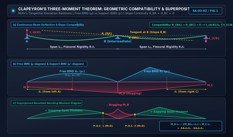
2.1 Geometric Compatibility at Intermediate Support BB

Because the beam is continuous and monolithic across support BB, the tangent to the elastic deflection curve must be continuous:

θBA+θBC=0\theta_{BA} + \theta_{BC} = 0

where θBA\theta_{BA} is the slope of tangent BABA at BB (measured relative to the chord ABAB), and θBC\theta_{BC} is the slope of tangent BCBC at BB (measured relative to chord BCBC).

Using Mohr's Second Moment-Area Theorem, the vertical deviation of support point AA from the tangent drawn to the elastic curve at BB is given by tA/Bt_{A/B}:

tA/B=∫0L1M(x)⋅xE1I1dxt_{A/B} = \int_0^{L_1} \frac{M(x) \cdot x}{E_1 I_1} dx

where xx is measured from the outer support AA.

Similarly, the vertical deviation of support point CC from the tangent drawn at BB is:

tC/B=∫0L2M(x)⋅xE2I2dxt_{C/B} = \int_0^{L_2} \frac{M(x) \cdot x}{E_2 I_2} dx

where xx is measured from the outer support CC.

Accounting for support settlements ΔA,ΔB,ΔC\Delta_A, \Delta_B, \Delta_C:

θBA=tA/B+ΔA−ΔBL1\theta_{BA} = \frac{t_{A/B} + \Delta_A - \Delta_B}{L_1} θBC=tC/B+ΔC−ΔBL2\theta_{BC} = \frac{t_{C/B} + \Delta_C - \Delta_B}{L_2}

Equating the slopes by compatibility (θBA+θBC=0\theta_{BA} + \theta_{BC} = 0):

tA/BL1+tC/BL2=−(ΔA−ΔBL1+ΔC−ΔBL2)\frac{t_{A/B}}{L_1} + \frac{t_{C/B}}{L_2} = - \left( \frac{\Delta_A - \Delta_B}{L_1} + \frac{\Delta_C - \Delta_B}{L_2} \right)

2.2 Decomposition of Bending Moment Diagram

By the principle of superposition, the total bending moment M(x)M(x) along each span is the algebraic sum of two independent components:

  1. Free Bending Moment (μ\mu-diagram): The bending moment produced by the external loads when each span is treated as a detached, simply supported beam.
  2. Support Bending Moment (μ′\mu'-diagram): The bending moment produced exclusively by the end support moments (MA,MBM_A, M_B on span 1; MB,MCM_B, M_C on span 2).

Free Bending Moment Area (AA) and Centroid (xˉ\bar{x})

  • Let A1A_1 = area of the simply supported free BMD on span ABAB.
  • Let xˉ1\bar{x}_1 = distance of the centroid of A1A_1 from the left support AA.
  • Let A2A_2 = area of the simply supported free BMD on span BCBC.
  • Let xˉ2\bar{x}_2 = distance of the centroid of A2A_2 from the right support CC.

The moment of the free BMD area about the outer supports is:

(tA/B)free=A1xˉ1E1I1,(tC/B)free=A2xˉ2E2I2(t_{A/B})_{\text{free}} = \frac{A_1 \bar{x}_1}{E_1 I_1}, \qquad (t_{C/B})_{\text{free}} = \frac{A_2 \bar{x}_2}{E_2 I_2}

Support Bending Moment Area (μ′\mu')

The support moment diagram on span ABAB is a trapezoid with ordinates MAM_A at AA and MBM_B at BB. Dividing this trapezoid into two triangles:

  • Triangle 1 (base L1L_1, height MAM_A): Area =12MAL1= \frac{1}{2} M_A L_1, centroid from A=13L1A = \frac{1}{3} L_1.
  • Triangle 2 (base L1L_1, height MBM_B): Area =12MBL1= \frac{1}{2} M_B L_1, centroid from A=23L1A = \frac{2}{3} L_1.

The moment of the support BMD area about AA is:

(tA/B)support=1E1I1[(12MAL1)(L13)+(12MBL1)(2L13)]=L126E1I1(MA+2MB)(t_{A/B})_{\text{support}} = \frac{1}{E_1 I_1} \left[ \left(\frac{1}{2} M_A L_1\right) \left(\frac{L_1}{3}\right) + \left(\frac{1}{2} M_B L_1\right) \left(\frac{2 L_1}{3}\right) \right] = \frac{L_1^2}{6 E_1 I_1} (M_A + 2 M_B)

Similarly, for span BCBC, measuring xx from CC:

(tC/B)support=1E2I2[(12MCL2)(L23)+(12MBL2)(2L23)]=L226E2I2(MC+2MB)(t_{C/B})_{\text{support}} = \frac{1}{E_2 I_2} \left[ \left(\frac{1}{2} M_C L_2\right) \left(\frac{L_2}{3}\right) + \left(\frac{1}{2} M_B L_2\right) \left(\frac{2 L_2}{3}\right) \right] = \frac{L_2^2}{6 E_2 I_2} (M_C + 2 M_B)

2.3 The Canonical Three-Moment Equation

Substituting the total tangential deviations tA/B=(tA/B)free+(tA/B)supportt_{A/B} = (t_{A/B})_{\text{free}} + (t_{A/B})_{\text{support}} and tC/B=(tC/B)free+(tC/B)supportt_{C/B} = (t_{C/B})_{\text{free}} + (t_{C/B})_{\text{support}} into the compatibility equation:

1L1[A1xˉ1E1I1+L126E1I1(MA+2MB)]+1L2[A2xˉ2E2I2+L226E2I2(MC+2MB)]=−(ΔA−ΔBL1+ΔC−ΔBL2)\frac{1}{L_1} \left[ \frac{A_1 \bar{x}_1}{E_1 I_1} + \frac{L_1^2}{6 E_1 I_1} (M_A + 2 M_B) \right] + \frac{1}{L_2} \left[ \frac{A_2 \bar{x}_2}{E_2 I_2} + \frac{L_2^2}{6 E_2 I_2} (M_C + 2 M_B) \right] = - \left( \frac{\Delta_A - \Delta_B}{L_1} + \frac{\Delta_C - \Delta_B}{L_2} \right)

Multiplying throughout by 66:

MA(L1E1I1)+2MB(L1E1I1+L2E2I2)+MC(L2E2I2)=−6A1xˉ1E1I1L1−6A2xˉ2E2I2L2−6(ΔA−ΔBL1+ΔC−ΔBL2)\boxed{ M_A \left(\frac{L_1}{E_1 I_1}\right) + 2 M_B \left(\frac{L_1}{E_1 I_1} + \frac{L_2}{E_2 I_2}\right) + M_C \left(\frac{L_2}{E_2 I_2}\right) = - \frac{6 A_1 \bar{x}_1}{E_1 I_1 L_1} - \frac{6 A_2 \bar{x}_2}{E_2 I_2 L_2} - 6 \left( \frac{\Delta_A - \Delta_B}{L_1} + \frac{\Delta_C - \Delta_B}{L_2} \right) }

2.4 Special Case: Homogeneous Material and Constant Cross-Section (EI=constantEI = \text{constant})

When the flexural rigidity EIEI is constant throughout both spans and the supports are rigid (no settlement, ΔA=ΔB=ΔC=0\Delta_A = \Delta_B = \Delta_C = 0):

MAL1+2MB(L1+L2)+MCL2=−6A1xˉ1L1−6A2xˉ2L2\boxed{ M_A L_1 + 2 M_B (L_1 + L_2) + M_C L_2 = - \frac{6 A_1 \bar{x}_1}{L_1} - \frac{6 A_2 \bar{x}_2}{L_2} }

[!IMPORTANT] Centroid Direction Protocol: In Clapeyron's equation, xˉ1\bar{x}_1 MUST be measured from the left-hand support AA, and xˉ2\bar{x}_2 MUST be measured from the right-hand support CC. Measuring both from the center support BB will invert the loading asymmetry and produce erroneous support moments!


3. Standard Loading Terms (6AxˉL\frac{6 A \bar{x}}{L}) Reference Table

Loading Type on Span LL Simply Supported Max Moment (Mmax⁡M_{\max}) Free BMD Area (AA) Centroid Distance (xˉ\bar{x}) Standard Loading Term 6AxˉL\frac{6 A \bar{x}}{L}
Uniformly Distributed Load (ww) wL28\frac{w L^2}{8} (Parabola) 23L(wL28)=wL312\frac{2}{3} L \left(\frac{w L^2}{8}\right) = \frac{w L^3}{12} L2\frac{L}{2} (Symmetric) 6L(wL312)(L2)=wL34\frac{6}{L} \left(\frac{w L^3}{12}\right) \left(\frac{L}{2}\right) = \mathbf{\frac{w L^3}{4}}
Central Concentrated Load (PP) PL4\frac{P L}{4} (Triangle) 12L(PL4)=PL28\frac{1}{2} L \left(\frac{P L}{4}\right) = \frac{P L^2}{8} L2\frac{L}{2} (Symmetric) 6L(PL28)(L2)=38PL2\frac{6}{L} \left(\frac{P L^2}{8}\right) \left(\frac{L}{2}\right) = \mathbf{\frac{3}{8} P L^2}
Eccentric Concentrated Load (PP at aa from left, bb from right) PabL\frac{P a b}{L} (Triangle) 12L(PabL)=Pab2\frac{1}{2} L \left(\frac{P a b}{L}\right) = \frac{P a b}{2} From Left: xˉ1=L+a3\bar{x}_1 = \frac{L + a}{3}
From Right: xˉ2=L+b3\bar{x}_2 = \frac{L + b}{3}
From Left: Pab(L+a)L\mathbf{\frac{P a b (L + a)}{L}}
From Right: Pab(L+b)L\mathbf{\frac{P a b (L + b)}{L}}
Symmetrical Triangular Load (Peak w0w_0 at midspan) w0L212\frac{w_0 L^2}{12} (Parabolic Apex) 12L(w0L212)×43=w0L312\frac{1}{2} L \left(\frac{w_0 L^2}{12}\right) \times \frac{4}{3} = \frac{w_0 L^3}{12} L2\frac{L}{2} (Symmetric) 516w0L3\mathbf{\frac{5}{16} w_0 L^3}
Linearly Increasing Load (00 at left to w0w_0 at right) w0L293\frac{w_0 L^2}{9 \sqrt{3}} (Cubic Curve) w0L324\frac{w_0 L^3}{24} From Left: xˉ1=815L\bar{x}_1 = \frac{8}{15} L
From Right: xˉ2=715L\bar{x}_2 = \frac{7}{15} L
From Left: 860w0L3=215w0L3\mathbf{\frac{8}{60} w_0 L^3} = \frac{2}{15} w_0 L^3
From Right: 760w0L3\mathbf{\frac{7}{60} w_0 L^3}
Pure Applied Couple (M0M_0 at distance aa from left) M0bL\frac{M_0 b}{L} and −M0aL-\frac{M_0 a}{L} Two opposing triangles From Left: xˉ1\bar{x}_1
From Right: xˉ2\bar{x}_2
From Left: M0L(3a2−L2)\mathbf{\frac{M_0}{L} (3a^2 - L^2)}
From Right: M0L(L2−3b2)\mathbf{\frac{M_0}{L} (L^2 - 3b^2)}

4. Engineering Diagrams & Visual Explanations

4.1 Geometric Derivation & BMD Superposition

The diagram below illustrates the continuous elastic curve, the common slope angle θB\theta_B, the tangential deviations tA/Bt_{A/B} and tC/Bt_{C/B}, and the graphical superposition of the free sagging moments (μ\mu) with the hogging support moments (μ′\mu').

Clapeyron's Three-Moment Theorem Derivation

4.2 Special Boundary Conditions: Fictitious Span & Support Sinking

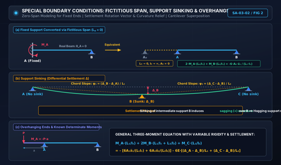
Fixed supports and differential settlements require specialized kinematic boundary modeling. The diagram below details:

  1. The fictitious zero-span model (L0→0,I0→∞L_0 \to 0, I_0 \to \infty) used to convert a fixed end into an equivalent continuous support.
  2. The settlement kinematic S-curve, proving why intermediate support sinking reduces hogging moment over that support while increasing midspan sagging moments.
  3. The cantilever overhang conversion, which transforms an overhanging span into an established, determinate boundary moment.
Fictitious Span and Support Sinking

5. Treatment of Boundary Conditions

5.1 Simply Supported / Roller Free Ends

If an end support (e.g., Support AA or Support CC) is a simple pin or roller support with no overhang:

Mend=0M_{\text{end}} = 0

This eliminates one unknown support moment immediately, leaving only the intermediate support moments to be computed.

5.2 Cantilever Overhangs

If the beam extends beyond an end support AA by an overhanging cantilever length aa subjected to a tip load PP and UDL ww:

MA=−(P⋅a+wa22)M_A = - \left( P \cdot a + \frac{w a^2}{2} \right)

The end support moment is statically determinate. It is substituted directly as a known numerical constant into the three-moment equation for the adjacent interior spans.

5.3 Fixed Ends (The Fictitious Zero-Span Method)

When an end of the continuous beam is clamped or fixed (e.g., fixed wall at AA), the slope of the elastic curve at AA is zero: θA=0\theta_A = 0. However, MA≠0M_A \ne 0 is an unknown fixed-end moment.

To generate the required additional equation without violating the three-support structure of Clapeyron's theorem:

  1. Introduce an imaginary fictitious span A0AA_0 A to the left of the fixed wall.
  2. Set length L0→0L_0 \to 0.
  3. Set second moment of area I0→∞I_0 \to \infty (or flexural rigidity E0I0→∞E_0 I_0 \to \infty).
  4. Because there are no loads on this imaginary span: A0=0A_0 = 0.

Applying Clapeyron's Three-Moment Equation to spans A0AA_0 A and ABAB:

M0(L0I0)+2MA(L0I0+L1I1)+MB(L1I1)=−6A0xˉ0L0I0−6A1xˉ1L1I1M_0 \left(\frac{L_0}{I_0}\right) + 2 M_A \left(\frac{L_0}{I_0} + \frac{L_1}{I_1}\right) + M_B \left(\frac{L_1}{I_1}\right) = - \frac{6 A_0 \bar{x}_0}{L_0 I_0} - \frac{6 A_1 \bar{x}_1}{L_1 I_1}

Substituting L0/I0=0L_0/I_0 = 0 and A0=0A_0 = 0:

2MA(L1I1)+MB(L1I1)=−6A1xˉ1L1I1\boxed{ 2 M_A \left(\frac{L_1}{I_1}\right) + M_B \left(\frac{L_1}{I_1}\right) = - \frac{6 A_1 \bar{x}_1}{L_1 I_1} }

[!TIP] Notice in this equation that xˉ1\bar{x}_1 is measured from the interior support BB toward AA! This linear equation provides the exact relation required to solve for the unknown fixed-end moment MAM_A.


6. Step-by-Step Analytical Procedure

To analyze any continuous beam using Clapeyron's Three-Moment Theorem, follow this systematic algorithm:

[Step 1: Determine Static Indeterminacy & Boundary Types]
  └─ Identify number of spans (m) and supports (n). Count unknown support moments.
  └─ If fixed end exists, add fictitious zero-span (L₀ = 0, I₀ = ∞).

[Step 2: Calculate Free BMD Quantities for Each Span]
  └─ Treat each span independently as simply supported.
  └─ Compute maximum free moment (wL²/8, PL/4, Pab/L).
  └─ Calculate free BMD area (A_i) and centroid distance (x̄_i).
  └─ Evaluate loading terms: 6A₁x̄₁/L₁ and 6A₂x̄₂/L₂.

[Step 3: Write Clapeyron's Three-Moment Equations]
  └─ Formulate one equation for each pair of adjacent spans across every intermediate support.
  └─ Incorporate settlement terms 6E·[(Δ_A - Δ_B)/L₁ + (Δ_C - Δ_B)/L₂] if supports sink.

[Step 4: Solve Simultaneous Linear Equations]
  └─ Solve for the unknown support moments M_A, M_B, M_C, ...

[Step 5: Compute Span Support Reactions via Static Equilibrium]
  └─ Separate each span as a free body:
     R_{AB} = R_{0,AB} + (M_A - M_B) / L₁
     R_{BA} = R_{0,BA} + (M_B - M_A) / L₁
  └─ Sum shears at common supports: R_B = R_{BA} + R_{BC}.

[Step 6: Construct Final SFD and Superposed BMD]
  └─ Locate points of zero shear: V(x) = 0.
  └─ Calculate maximum span sagging moments: M_max = M(x_0).
  └─ Find points of contraflexure where net M(x) = 0.

7. Solved Numerical Examples

Example 1: Two-Span Continuous Beam with Combined UDL and Central Point Load

Problem Statement:
A continuous beam ABCABC rests on three simple supports at A,BA, B, and CC at the same level.

  • Span AB=L1=6.0 mAB = L_1 = 6.0\text{ m} carries a uniformly distributed load of w=20 kN/mw = 20\text{ kN/m}.
  • Span BC=L2=4.0 mBC = L_2 = 4.0\text{ m} carries a central concentrated point load of P=40 kNP = 40\text{ kN} at midspan.
  • The flexural rigidity EIEI is constant throughout both spans.

Determine:

  1. Support moment at intermediate support BB.
  2. All vertical support reactions RA,RB,RCR_A, R_B, R_C.
  3. Maximum positive span bending moments and their locations.
  4. Points of contraflexure in both spans.
          20 kN/m                        40 kN
  ┌───────────────────────┐                ↓
  ▼ ▼ ▼ ▼ ▼ ▼ ▼ ▼ ▼ ▼ ▼ ▼ │         2 m    │    2 m
 [▲]─────────────────────[▲]───────────────┴───────────────[▲]
  A       L₁ = 6 m        B            L₂ = 4 m             C

Solution:

Step 1: Identify boundary conditions
Supports AA and CC are simply supported ends:

MA=0,MC=0M_A = 0, \qquad M_C = 0

The only unknown is the intermediate support moment MBM_B (Ds=1D_s = 1).

Step 2: Calculate Free BMD loading terms

  • Span ABAB (UDL):
    Free moment is parabolic with maximum height Mmax⁡,1=w1L128=20×628=90.0 kN⋅mM_{\max,1} = \frac{w_1 L_1^2}{8} = \frac{20 \times 6^2}{8} = 90.0\text{ kN}\cdot\text{m}.
    Area A1=23×L1×Mmax⁡,1=23×6×90=360 kN⋅m2A_1 = \frac{2}{3} \times L_1 \times M_{\max,1} = \frac{2}{3} \times 6 \times 90 = 360\text{ kN}\cdot\text{m}^2.
    By symmetry, the centroid from left support AA is xˉ1=L12=3.0 m\bar{x}_1 = \frac{L_1}{2} = 3.0\text{ m}.

    6A1xˉ1L1=w1L134=20×634=1080.0 kN⋅m2\frac{6 A_1 \bar{x}_1}{L_1} = \frac{w_1 L_1^3}{4} = \frac{20 \times 6^3}{4} = 1080.0\text{ kN}\cdot\text{m}^2
  • Span BCBC (Central Point Load):
    Free moment is triangular with peak at midspan Mmax⁡,2=PL24=40×44=40.0 kN⋅mM_{\max,2} = \frac{P L_2}{4} = \frac{40 \times 4}{4} = 40.0\text{ kN}\cdot\text{m}.
    Area A2=12×L2×Mmax⁡,2=12×4×40=80 kN⋅m2A_2 = \frac{1}{2} \times L_2 \times M_{\max,2} = \frac{1}{2} \times 4 \times 40 = 80\text{ kN}\cdot\text{m}^2.
    By symmetry, centroid from right support CC is xˉ2=L22=2.0 m\bar{x}_2 = \frac{L_2}{2} = 2.0\text{ m}.

    6A2xˉ2L2=38PL22=38×40×42=240.0 kN⋅m2\frac{6 A_2 \bar{x}_2}{L_2} = \frac{3}{8} P L_2^2 = \frac{3}{8} \times 40 \times 4^2 = 240.0\text{ kN}\cdot\text{m}^2

Step 3: Apply Clapeyron's Three-Moment Equation at support BB

MAL1+2MB(L1+L2)+MCL2=−6A1xˉ1L1−6A2xˉ2L2M_A L_1 + 2 M_B (L_1 + L_2) + M_C L_2 = - \frac{6 A_1 \bar{x}_1}{L_1} - \frac{6 A_2 \bar{x}_2}{L_2}

Substitute known values (MA=0,MC=0,L1=6,L2=4M_A = 0, M_C = 0, L_1 = 6, L_2 = 4):

0+2MB(6+4)+0=−(1080.0+240.0)0 + 2 M_B (6 + 4) + 0 = - (1080.0 + 240.0) 20MB=−1320.0  ⟹  MB=−66.0 kN⋅m20 M_B = - 1320.0 \implies M_B = -66.0\text{ kN}\cdot\text{m}

The negative sign confirms that MBM_B is a hogging bending moment of magnitude 66.0 kN⋅m66.0\text{ kN}\cdot\text{m}.

Step 4: Compute Support Reactions
Analyze each span as an independent free body:

  • Span ABAB (L1=6 mL_1 = 6\text{ m}):
    Taking moments about BB:

    ∑MB=0  ⟹  RA×6−20×622+MB=0\sum M_B = 0 \implies R_A \times 6 - \frac{20 \times 6^2}{2} + M_B = 0 6RA−360−66.0=0  ⟹  6RA=294.0  ⟹  RA=49.0 kN6 R_A - 360 - 66.0 = 0 \implies 6 R_A = 294.0 \implies \mathbf{R_A = 49.0\text{ kN}}

    Vertical equilibrium of span ABAB:

    RBA=20×6−RA=120−49.0=71.0 kNR_{BA} = 20 \times 6 - R_A = 120 - 49.0 = \mathbf{71.0\text{ kN}}
  • Span BCBC (L2=4 mL_2 = 4\text{ m}):
    Taking moments about BB:

    ∑MB=0  ⟹  RC×4−40×2+MB=0\sum M_B = 0 \implies R_C \times 4 - 40 \times 2 + M_B = 0 4RC−80−66.0=0  ⟹  4RC=14.0  ⟹  RC=3.5 kN4 R_C - 80 - 66.0 = 0 \implies 4 R_C = 14.0 \implies \mathbf{R_C = 3.5\text{ kN}}

    Vertical equilibrium of span BCBC:

    RBC=40−RC=40−3.5=36.5 kNR_{BC} = 40 - R_C = 40 - 3.5 = \mathbf{36.5\text{ kN}}
  • Total Intermediate Support Reaction RBR_B:

    RB=RBA+RBC=71.0+36.5=107.5 kNR_B = R_{BA} + R_{BC} = 71.0 + 36.5 = \mathbf{107.5\text{ kN}}

Equilibrium Check:

∑Fy=RA+RB+RC=49.0+107.5+3.5=160.0 kN\sum F_y = R_A + R_B + R_C = 49.0 + 107.5 + 3.5 = 160.0\text{ kN} Total applied load=(20×6)+40=160.0 kN[EXACT MATCH]\text{Total applied load} = (20 \times 6) + 40 = 160.0\text{ kN} \quad \text{[EXACT MATCH]}

Step 5: Maximum Span Sagging Moments & Points of Contraflexure

  • Span ABAB:
    Shear force at distance xx from AA: V(x)=RA−wx=49.0−20xV(x) = R_A - w x = 49.0 - 20 x.
    Zero shear location: 49.0−20x0=0  ⟹  x0=2.45 m49.0 - 20 x_0 = 0 \implies x_0 = \mathbf{2.45\text{ m}} from AA.

    Mmax⁡,AB=RAx0−wx022=49.0(2.45)−20(2.45)22=120.05−60.025=+60.025 kN⋅mM_{\max, AB} = R_A x_0 - \frac{w x_0^2}{2} = 49.0(2.45) - \frac{20(2.45)^2}{2} = 120.05 - 60.025 = \mathbf{+60.025\text{ kN}\cdot\text{m}}

    Point of Contraflexure (M(x)=0M(x) = 0):

    49.0x−10x2=0  ⟹  x(49.0−10x)=0  ⟹  xc=49.010=4.90 m from A (1.10 m from B)49.0 x - 10 x^2 = 0 \implies x(49.0 - 10 x) = 0 \implies x_c = \frac{49.0}{10} = \mathbf{4.90\text{ m}}\text{ from } A \text{ ($1.10\text{ m}$ from } B\text{)}
  • Span BCBC:
    Shear force changes sign at midspan under the 40 kN40\text{ kN} load (x=2 mx = 2\text{ m} from CC).
    Bending moment under load (2 m2\text{ m} from CC):

    M(2 m)=RC×2=3.5×2=+7.0 kN⋅mM(2\text{ m}) = R_C \times 2 = 3.5 \times 2 = \mathbf{+7.0\text{ kN}\cdot\text{m}}

    Point of Contraflexure in span BCBC (xx measured from CC, for x>2 mx > 2\text{ m}):

    M(x)=RCx−40(x−2)=0  ⟹  3.5x−40x+80=0  ⟹  36.5x=80  ⟹  xc=2.192 m from C (1.808 m from B)M(x) = R_C x - 40(x - 2) = 0 \implies 3.5 x - 40 x + 80 = 0 \implies 36.5 x = 80 \implies x_c = \mathbf{2.192\text{ m}}\text{ from } C \text{ ($1.808\text{ m}$ from } B\text{)}

Example 2: Continuous Beam with Fixed End at Support AA (Fictitious Span Application)

Problem Statement:
A two-span continuous beam ABCABC is built-in (fixed) at support AA, continuous over simple roller support BB, and simply supported at CC.

  • Span AB=L1=6.0 mAB = L_1 = 6.0\text{ m} carries a uniformly distributed load of w=18 kN/mw = 18\text{ kN/m}.
  • Span BC=L2=5.0 mBC = L_2 = 5.0\text{ m} carries an eccentric concentrated load of P=50 kNP = 50\text{ kN} located at 2.0 m2.0\text{ m} from support BB (3.0 m3.0\text{ m} from support CC).
  • Flexural rigidity EIEI is uniform throughout.

Calculate:

  1. The fixed-end moment MAM_A and intermediate support moment MBM_B.
  2. All vertical support reactions.
  3. Maximum span bending moment in span ABAB.
   Fixed                18 kN/m                       50 kN
  ┌──┐         ┌───────────────────────┐                ↓
  │  │         ▼ ▼ ▼ ▼ ▼ ▼ ▼ ▼ ▼ ▼ ▼ ▼ │         2 m    │     3 m
  │  │[▲]─────────────────────────────[▲]───────────────┴───────────────[▲]
  └──┘ A              L₁ = 6 m         B             L₂ = 5 m            C

Solution:

Step 1: Setup Fictitious Span A0AA_0 A for the Fixed Support at AA
Introduce an imaginary zero-span A0AA_0 A with L0=0,I0=∞,A0=0L_0 = 0, I_0 = \infty, A_0 = 0.
Support CC is simply supported: MC=0M_C = 0.
Unknowns: MAM_A and MBM_B (Ds=2D_s = 2).

Step 2: Evaluate Free BMD Loading Terms

  • Span ABAB (UDL):

    6A1xˉ1L1=w1L134=18×634=972.0 kN⋅m2\frac{6 A_1 \bar{x}_1}{L_1} = \frac{w_1 L_1^3}{4} = \frac{18 \times 6^3}{4} = 972.0\text{ kN}\cdot\text{m}^2

    Because the load is symmetric, the term is identical whether xˉ1\bar{x}_1 is measured from AA or from BB.

  • Span BCBC (Eccentric point load P=50 kN,a=2 mP = 50\text{ kN}, a = 2\text{ m} from B,b=3 mB, b = 3\text{ m} from CC):
    Free BMD area A2=Pab2=50×2×32=150 kN⋅m2A_2 = \frac{P a b}{2} = \frac{50 \times 2 \times 3}{2} = 150\text{ kN}\cdot\text{m}^2.
    Centroid from right support CC: xˉ2=L2+b3=5+33=83 m\bar{x}_2 = \frac{L_2 + b}{3} = \frac{5 + 3}{3} = \frac{8}{3}\text{ m}.

    6A2xˉ2L2=Pab(L2+b)L2=50×2×3×(5+3)5=300×85=480.0 kN⋅m2\frac{6 A_2 \bar{x}_2}{L_2} = \frac{P a b (L_2 + b)}{L_2} = \frac{50 \times 2 \times 3 \times (5 + 3)}{5} = \frac{300 \times 8}{5} = 480.0\text{ kN}\cdot\text{m}^2

Step 3: Equation 1 — Clapeyron's Equation for Spans A0AA_0 A and ABAB (at Support AA)

M0L0+2MA(L0+L1)+MBL1=−6A0xˉ0L0−6A1xˉ1L1M_0 L_0 + 2 M_A (L_0 + L_1) + M_B L_1 = - \frac{6 A_0 \bar{x}_0}{L_0} - \frac{6 A_1 \bar{x}_1}{L_1}

Substituting L0=0L_0 = 0 and A0=0A_0 = 0:

2MA(0+6)+MB(6)=−972.02 M_A (0 + 6) + M_B (6) = - 972.0 12MA+6MB=−972.0  ⟹  2MA+MB=−162.0— (Eq. 1)12 M_A + 6 M_B = - 972.0 \implies 2 M_A + M_B = - 162.0 \quad \text{--- (Eq. 1)}

Step 4: Equation 2 — Clapeyron's Equation for Spans ABAB and BCBC (at Support BB)

MAL1+2MB(L1+L2)+MCL2=−6A1xˉ1L1−6A2xˉ2L2M_A L_1 + 2 M_B (L_1 + L_2) + M_C L_2 = - \frac{6 A_1 \bar{x}_1}{L_1} - \frac{6 A_2 \bar{x}_2}{L_2}

Substitute MC=0,L1=6,L2=5M_C = 0, L_1 = 6, L_2 = 5:

6MA+2MB(6+5)+0=−(972.0+480.0)6 M_A + 2 M_B (6 + 5) + 0 = - (972.0 + 480.0) 6MA+22MB=−1452.0  ⟹  3MA+11MB=−726.0— (Eq. 2)6 M_A + 22 M_B = - 1452.0 \implies 3 M_A + 11 M_B = - 726.0 \quad \text{--- (Eq. 2)}

Step 5: Solve the System of Simultaneous Equations
From Eq. (1):

MB=−162.0−2MAM_B = -162.0 - 2 M_A

Substitute into Eq. (2):

3MA+11(−162.0−2MA)=−726.03 M_A + 11 (-162.0 - 2 M_A) = -726.0 3MA−1782.0−22MA=−726.03 M_A - 1782.0 - 22 M_A = -726.0 −19MA=1056.0  ⟹  MA=−105619≈−55.579 kN⋅m-19 M_A = 1056.0 \implies \mathbf{M_A = -\frac{1056}{19} \approx -55.579\text{ kN}\cdot\text{m}}

Now solve for MBM_B:

MB=−162.0−2(−55.5789)=−162.0+111.1579=−50.842 kN⋅mM_B = -162.0 - 2(-55.5789) = -162.0 + 111.1579 = \mathbf{-50.842\text{ kN}\cdot\text{m}}

Both MAM_A and MBM_B are hogging moments (∣MA∣=55.58 kN⋅m|M_A| = 55.58\text{ kN}\cdot\text{m}, ∣MB∣=50.84 kN⋅m|M_B| = 50.84\text{ kN}\cdot\text{m}).

Step 6: Calculate Vertical Reactions

  • Span ABAB (L1=6 mL_1 = 6\text{ m}):
    Taking moments about BB:

    RA×6−18×622+MA−MB=0R_A \times 6 - \frac{18 \times 6^2}{2} + M_A - M_B = 0 6RA=324.0+MB−MA=324.0+(−50.8421)−(−55.5789)=324.0+4.7368=328.73686 R_A = 324.0 + M_B - M_A = 324.0 + (-50.8421) - (-55.5789) = 324.0 + 4.7368 = 328.7368 RA=54.789 kN\mathbf{R_A = 54.789\text{ kN}} RBA=18×6−54.7895=53.211 kNR_{BA} = 18 \times 6 - 54.7895 = \mathbf{53.211\text{ kN}}
  • Span BCBC (L2=5 mL_2 = 5\text{ m}):
    Taking moments about BB:

    RC×5−50×2+MB=0  ⟹  5RC=100.0−50.8421=49.1579R_C \times 5 - 50 \times 2 + M_B = 0 \implies 5 R_C = 100.0 - 50.8421 = 49.1579 RC=9.832 kN\mathbf{R_C = 9.832\text{ kN}} RBC=50−9.8316=40.168 kNR_{BC} = 50 - 9.8316 = \mathbf{40.168\text{ kN}}
  • Total Reaction at Support BB:

    RB=RBA+RBC=53.2105+40.1684=93.379 kNR_B = R_{BA} + R_{BC} = 53.2105 + 40.1684 = \mathbf{93.379\text{ kN}}

Equilibrium Check:

RA+RB+RC=54.7895+93.3789+9.8316=158.000 kNR_A + R_B + R_C = 54.7895 + 93.3789 + 9.8316 = 158.000\text{ kN} Total applied load=(18×6)+50=158.0 kN[EXACT MATCH]\text{Total applied load} = (18 \times 6) + 50 = 158.0\text{ kN} \quad \text{[EXACT MATCH]}

Step 7: Maximum Span Sagging Moment in Span ABAB
Zero shear location in span ABAB:

V(x)=RA−18x=0  ⟹  x0=54.789518=3.044 m from AV(x) = R_A - 18 x = 0 \implies x_0 = \frac{54.7895}{18} = \mathbf{3.044\text{ m}}\text{ from } A Mmax⁡,AB=MA+RAx0−18x022=−55.5789+54.7895(3.0439)−9(3.0439)2M_{\max, AB} = M_A + R_A x_0 - \frac{18 x_0^2}{2} = -55.5789 + 54.7895(3.0439) - 9(3.0439)^2 Mmax⁡,AB=−55.5789+166.7738−83.3881=+27.807 kN⋅mM_{\max, AB} = -55.5789 + 166.7738 - 83.3881 = \mathbf{+27.807\text{ kN}\cdot\text{m}}

Example 3: Effect of Support Settlement (Differential Sinking)

Problem Statement:
A continuous beam ABCABC is supported on simple supports at A,BA, B, and CC.

  • Span AB=L1=8.0 mAB = L_1 = 8.0\text{ m}, carrying a UDL of w1=15 kN/mw_1 = 15\text{ kN/m}.
  • Span BC=L2=6.0 mBC = L_2 = 6.0\text{ m}, carrying a UDL of w2=20 kN/mw_2 = 20\text{ kN/m}.
  • Flexural rigidity EI=60,000 kN⋅m2EI = 60,000\text{ kN}\cdot\text{m}^2 is constant.

Evaluate the intermediate support moment MBM_B and reactions for two scenarios:

  1. Case (a): All supports are unyielding (rigid).
  2. Case (b): Intermediate support BB settles (sinks) downward by ΔB=10 mm=0.010 m\Delta_B = 10\text{ mm} = 0.010\text{ m}.

Solution:

Step 1: Free BMD Loading Terms

  • Span ABAB: 6A1xˉ1L1=w1L134=15×834=1920.0 kN⋅m2\frac{6 A_1 \bar{x}_1}{L_1} = \frac{w_1 L_1^3}{4} = \frac{15 \times 8^3}{4} = 1920.0\text{ kN}\cdot\text{m}^2
  • Span BCBC: 6A2xˉ2L2=w2L234=20×634=1080.0 kN⋅m2\frac{6 A_2 \bar{x}_2}{L_2} = \frac{w_2 L_2^3}{4} = \frac{20 \times 6^3}{4} = 1080.0\text{ kN}\cdot\text{m}^2

Step 2: Case (a) — Rigid Supports (No Settlement)
Because ends AA and CC are simply supported: MA=0,MC=0M_A = 0, M_C = 0.

MAL1+2MB(L1+L2)+MCL2=−(1920.0+1080.0)M_A L_1 + 2 M_B (L_1 + L_2) + M_C L_2 = - (1920.0 + 1080.0) 2MB(8+6)=−3000.0  ⟹  28MB=−3000.02 M_B (8 + 6) = - 3000.0 \implies 28 M_B = - 3000.0 MB=−107.143 kN⋅m(Hogging moment)\mathbf{M_B = -107.143\text{ kN}\cdot\text{m}} \quad \text{(Hogging moment)}

Support Reactions for Case (a):

  • Span ABAB: RA=15×82/2+MB8=480−107.1438=46.607 kNR_A = \frac{15 \times 8^2 / 2 + M_B}{8} = \frac{480 - 107.143}{8} = \mathbf{46.607\text{ kN}}, RBA=120−46.607=73.393 kNR_{BA} = 120 - 46.607 = 73.393\text{ kN}.
  • Span BCBC: RC=20×62/2+MB6=360−107.1436=42.143 kNR_C = \frac{20 \times 6^2 / 2 + M_B}{6} = \frac{360 - 107.143}{6} = \mathbf{42.143\text{ kN}}, RBC=120−42.143=77.857 kNR_{BC} = 120 - 42.143 = 77.857\text{ kN}.
  • Reaction RB=73.393+77.857=151.250 kNR_B = 73.393 + 77.857 = \mathbf{151.250\text{ kN}}.

Step 3: Case (b) — Support BB Sinks by ΔB=10 mm=0.010 m\Delta_B = 10\text{ mm} = 0.010\text{ m}
Settlements: ΔA=0,ΔB=0.010 m,ΔC=0\Delta_A = 0, \Delta_B = 0.010\text{ m}, \Delta_C = 0.
Evaluate the settlement term:

Settlement Term=−6E[ΔA−ΔBL1+ΔC−ΔBL2]\text{Settlement Term} = - 6 E \left[ \frac{\Delta_A - \Delta_B}{L_1} + \frac{\Delta_C - \Delta_B}{L_2} \right] −6EI[0−0.0108+0−0.0106]=−6(60,000)[−0.0108−0.0106]- 6 EI \left[ \frac{0 - 0.010}{8} + \frac{0 - 0.010}{6} \right] = - 6 (60,000) \left[ - \frac{0.010}{8} - \frac{0.010}{6} \right] =+360,000×0.010(18+16)=3600×(724)=+1050.0 kN⋅m2= + 360,000 \times 0.010 \left( \frac{1}{8} + \frac{1}{6} \right) = 3600 \times \left( \frac{7}{24} \right) = \mathbf{+1050.0\text{ kN}\cdot\text{m}^2}

Notice the positive sign! Sinking of support BB counteracts the negative loading terms.

Now write the full three-moment equation:

28MB=−(1920.0+1080.0)+1050.0=−3000.0+1050.0=−1950.028 M_B = - (1920.0 + 1080.0) + 1050.0 = - 3000.0 + 1050.0 = - 1950.0 MB=−1950.028≈−69.643 kN⋅m\mathbf{M_B = - \frac{1950.0}{28} \approx -69.643\text{ kN}\cdot\text{m}}

Step 4: Comparative Engineering Assessment

Structural Response Parameter Case (a): Rigid Supports Case (b): Support BB Sinks 10 mm10\text{ mm} Percentage Change
Intermediate Support Moment MBM_B −107.143 kN⋅m-107.143\text{ kN}\cdot\text{m} −69.643 kN⋅m-69.643\text{ kN}\cdot\text{m} −35.0%-35.0\% (Hogging Relieved)
Left End Reaction RAR_A 46.607 kN46.607\text{ kN} 51.295 kN51.295\text{ kN} +10.1%+10.1\%
Intermediate Support Reaction RBR_B 151.250 kN151.250\text{ kN} 140.312 kN140.312\text{ kN} −7.2%-7.2\% (Load Shed to Ends)
Right End Reaction RCR_C 42.143 kN42.143\text{ kN} 48.393 kN48.393\text{ kN} +14.8%+14.8\%
Max Sagging Moment (Span ABAB) +72.41 kN⋅m+72.41\text{ kN}\cdot\text{m} +87.70 kN⋅m+87.70\text{ kN}\cdot\text{m} +21.1%+21.1\% (Severe Increase!)

[!CAUTION] While sinking of an interior pier reduces the hogging moment directly over it, it forces the spans to carry additional sagging moment (+21.1%+21.1\% in span ABAB). If a bridge girder was not designed for this increased positive midspan moment, settlement can induce severe flexural cracking or bottom flange failure!


8. Practical Applications & Design Codes (IS 456 & IS 800)

8.1 Moment Redistribution in Reinforced Concrete (IS 456:2000 Clause 37.1)

Continuous reinforced concrete beams analyzed by elastic methods (such as Clapeyron's theorem) exhibit high hogging moment peaks over supports. Under ultimate load conditions, high plastic rotation capacity at supports permits moment redistribution:

  • According to IS 456:2000 Clause 37.1.1, elastic moments may be redistributed by up to 30%30\%, provided that: βb≥xud+% redistribution100\beta_b \ge \frac{x_u}{d} + \frac{\% \text{ redistribution}}{100} where xu/d≤0.48x_u/d \le 0.48 (for Fe 415 steel) to ensure ductile behavior before yielding.
  • When support moments are reduced by redistribution, span sagging moments must be increased proportionally to maintain static equilibrium across each span.

8.2 Deflection Control in Continuous Beams (IS 456 Clause 23.2.1)

The basic span-to-effective-depth ratio (L/dL/d) for continuous beams is significantly more relaxed than for simply supported beams:

  • Simply Supported: Basic Ld=20\frac{L}{d} = 20.
  • Cantilever: Basic Ld=7\frac{L}{d} = 7.
  • Continuous Beam: Basic Ld=26\mathbf{\frac{L}{d} = 26}.

The continuity reduces deflections, enabling much more slender and economical floor systems.


9. Comparative Matrix: Classical Methods of Indeterminate Beam Analysis

Feature / Criteria Clapeyron's Three-Moment Theorem Slope-Deflection Method Moment Distribution Method (Hardy Cross) Flexibility Matrix Method
Primary Classification Force Method (Compatibility) Displacement Method Displacement (Iterative Relaxation) Force Method (Matrix Formulation)
Primary Unknowns Support Moments (MiM_i) Joint Rotations (θi\theta_i) & Sway (Δ\Delta) Unbalanced Joint Moments Redundant Forces / Moments ({X}\{X\})
Equation Type Three-term linear recurrence Simultaneous linear equations Successive cycle approximation System of matrix equations [F]{X}={Δ}[F]\{X\} = \{\Delta\}
Best Suited For Multi-span continuous beams Rigid portal frames, non-sway frames Hand calculation of complex continuous beams Computational analysis of large frames/trusses
Handling Fixed Supports Requires fictitious zero-span (L0=0L_0 = 0) Naturally incorporated (θfixed=0\theta_{\text{fixed}} = 0) Fixed End Moments (FEMs) directly locked Select fixed reaction as redundant force
Support Settlement Directly added via 6E[(ΔA−ΔB)/L]6E[(\Delta_A-\Delta_B)/L] Added via chord rotation term ψ=Δ/L\psi = \Delta/L Handled via initial settlement FEMs (6EIΔ/L26EI\Delta/L^2) Direct displacement vector {Δ0}\{\Delta_0\}

10. Common Misconceptions & Exam Traps

[!WARNING]

1. Centroid Measurement Inversion

Misconception: Measuring both centroids xˉ1\bar{x}_1 and xˉ2\bar{x}_2 from the middle support BB.
Reality: The derivation of Clapeyron's theorem relies on tangential deviations taken from the outer supports AA and CC. Therefore, xˉ1\bar{x}_1 MUST be measured from the left support AA, and xˉ2\bar{x}_2 MUST be measured from the right support CC. Measuring from BB gives the wrong answer for any asymmetric load!

[!WARNING]

2. The Fictitious Span Parameter Error

Misconception: Setting I0→0I_0 \to 0 for the fictitious zero span at a fixed end.
Reality: Setting I0→0I_0 \to 0 makes flexural stiffness zero (a hinge). To model a perfectly rigid fixed support (θ=0\theta = 0), the fictitious span must be infinitely stiff: I0→∞I_0 \to \infty (so L0/I0→0L_0/I_0 \to 0).

[!WARNING]

3. Intermediate Support Reaction Calculation

Misconception: Calculating the reaction at continuous support BB simply as the sum of free simply supported reactions (RB=R0,BA+R0,BCR_B = R_{0,BA} + R_{0,BC}).
Reality: The support moments MA,MB,MCM_A, M_B, M_C create internal couples that significantly alter the shear forces. The correct reaction is:

RB=(R0,BA+MB−MAL1)+(R0,BC+MB−MCL2)R_B = \left( R_{0,BA} + \frac{M_B - M_A}{L_1} \right) + \left( R_{0,BC} + \frac{M_B - M_C}{L_2} \right)

[!WARNING]

4. Sinking Sign Convention

Misconception: Sinking of an intermediate support always increases stress.
Reality: Sinking of an intermediate support BB relieves (reduces) the hogging moment over BB. However, this relief causes a dangerous increase in the midspan sagging moments in both adjacent spans!


11. Practice Problems

Problem 1 (GATE CE Standard)

A continuous beam ABCABC has two equal spans L1=L2=6 mL_1 = L_2 = 6\text{ m} of uniform flexural rigidity EIEI. Supports AA and CC are simple. The beam carries a uniformly distributed load of w=12 kN/mw = 12\text{ kN/m} over the entire length.

  1. Determine the hogging bending moment at intermediate support BB.
  2. Calculate the vertical reaction at support BB.
  3. Find the location of the points of contraflexure measured from support BB.

Answer:

  1. MB=−54.0 kN⋅mM_B = -54.0\text{ kN}\cdot\text{m}.
  2. RB=90.0 kNR_B = 90.0\text{ kN}, RA=RC=27.0 kNR_A = R_C = 27.0\text{ kN}.
  3. xc=1.50 mx_c = 1.50\text{ m} from BB in each span (4.50 m4.50\text{ m} from outer supports).

Problem 2 (UPSC ESE Conventional Standard)

A continuous beam ABCDABCD covers three spans: AB=4 m,BC=6 m,CD=4 mAB = 4\text{ m}, BC = 6\text{ m}, CD = 4\text{ m}, supported on simple supports at A,B,C,DA, B, C, D.

  • Span ABAB carries a central concentrated load of 40 kN40\text{ kN}.
  • Span BCBC carries a UDL of 20 kN/m20\text{ kN/m}.
  • Span CDCD carries a central concentrated load of 40 kN40\text{ kN}.
  • Rigidity EIEI is constant throughout.

Using Clapeyron's Three-Moment Theorem, determine support moments MBM_B and MCM_C, and draw the bending moment diagram showing key ordinates.

Answer:
By symmetry, MB=MCM_B = M_C.
Applying three-moment theorem on spans ABAB and BCBC:
4(0)+2MB(4+6)+6MC=−38(40)(42)−20(63)44(0) + 2 M_B (4 + 6) + 6 M_C = - \frac{3}{8}(40)(4^2) - \frac{20(6^3)}{4}
20MB+6MB=26MB=−(240+1080)=−1320  ⟹  MB=MC=−50.77 kN⋅m20 M_B + 6 M_B = 26 M_B = - (240 + 1080) = -1320 \implies \mathbf{M_B = M_C = -50.77\text{ kN}\cdot\text{m}}.


12. Quick Revision Formula Summary

General Form:MA(L1I1)+2MB(L1I1+L2I2)+MC(L2I2)=−(6A1xˉ1L1I1+6A2xˉ2L2I2)−6E(ΔA−ΔBL1+ΔC−ΔBL2)Uniform EI (Rigid):MAL1+2MB(L1+L2)+MCL2=−6A1xˉ1L1−6A2xˉ2L2UDL Loading Term:6AxˉL=wL34Central Point Load Term:6AxˉL=38PL2Eccentric Point Load Term:6A1xˉ1L=Pab(L+a)L(xˉ1 from left)Fixed End Conversion:L0=0,I0=∞  ⟹  2MA(L1I1)+MB(L1I1)=−6A1xˉ1L1I1\begin{aligned} \text{General Form:} \quad & M_A \left(\frac{L_1}{I_1}\right) + 2 M_B \left(\frac{L_1}{I_1} + \frac{L_2}{I_2}\right) + M_C \left(\frac{L_2}{I_2}\right) \\ &= - \left( \frac{6 A_1 \bar{x}_1}{L_1 I_1} + \frac{6 A_2 \bar{x}_2}{L_2 I_2} \right) - 6E \left( \frac{\Delta_A - \Delta_B}{L_1} + \frac{\Delta_C - \Delta_B}{L_2} \right) \\[10pt] \text{Uniform } EI \text{ (Rigid):} \quad & M_A L_1 + 2 M_B (L_1 + L_2) + M_C L_2 = - \frac{6 A_1 \bar{x}_1}{L_1} - \frac{6 A_2 \bar{x}_2}{L_2} \\[10pt] \text{UDL Loading Term:} \quad & \frac{6 A \bar{x}}{L} = \frac{w L^3}{4} \\[10pt] \text{Central Point Load Term:} \quad & \frac{6 A \bar{x}}{L} = \frac{3}{8} P L^2 \\[10pt] \text{Eccentric Point Load Term:} \quad & \frac{6 A_1 \bar{x}_1}{L} = \frac{P a b (L + a)}{L} \quad (\bar{x}_1 \text{ from left}) \\[10pt] \text{Fixed End Conversion:} \quad & L_0 = 0, \quad I_0 = \infty \implies 2 M_A \left(\frac{L_1}{I_1}\right) + M_B \left(\frac{L_1}{I_1}\right) = - \frac{6 A_1 \bar{x}_1}{L_1 I_1} \end{aligned}