Stiffness Method (Displacement & Direct Assembly)
In this chapter (4 topics)
On this page
- 1. Introduction & Executive Overview
- Core Axioms of the Stiffness Formulation
- 2. Fundamentals & Physical Mechanics
- 2.1 Degrees of Freedom & Kinematic Indeterminacy (Dk)
- 2.2 Physical Interpretation of Stiffness Coefficients
- 3. Mathematical Derivations & Theoretical Formulations
- 3.1 Prismatic Flexural Beam Element (Euler-Bernoulli Beam)
- 3.2 2D Pin-Jointed Truss Element & Coordinate Transformation
- 3.3 The Direct Stiffness Assembly Algorithm
- 3.4 Load Vector Assembly & Support Settlement
- 4. Engineering Diagrams & Visual Explanations
- Figure 1: Direct Stiffness Method — Kinematic Locking & Assembly
- Figure 2: Element Stiffness Matrices & Coordinate Transformations
- 5. Practical Engineering Applications & Software Implementations
- 6. Comparative Analysis Table
- 7. Worked Numerical Examples
- Problem 1: Continuous Beam ABC — Exact Dual Verification with Flexibility Method
- Problem 2: 2D Planar Truss Analysis via Coordinate Transformation
- Problem 3: Propped Cantilever Subjected to Downward Support Settlement
- 8. Exam-Oriented Traps, Common Errors & Misconceptions
- 9. Competitive Examination Key Points & Memory Triggers
- 10. Previous Year & Model Examination Questions
- Question 1 (GATE CE)
- Question 2 (UPSC ESE)
- Question 3 (SSC JE / State AE)
- 11. Summary & Quick Revision Formula Sheet
- 12. References & Standard Code Provisions
1. Introduction & Executive Overview
The Stiffness Method—also universally designated as the Displacement Method or Direct Stiffness Method (DSM)—is the foundational computational engine underpinning modern structural engineering and Finite Element Analysis (FEA) software (including ETABS, SAP2000, STAAD.Pro, and ANSYS). While the Flexibility (Force) Method selects internal redundant forces () as unknowns, the Stiffness Method treats the unknown joint displacements—translations and rotations ()—as primary unknowns.
The formulation begins from a kinematically locked base system, where every free degree of freedom is artificially clamped (). External member loads generate fixed-end holding forces and moments (). The artificial clamps are then systematically released, allowing the structure to deform into its true equilibrium state under the action of net unbalanced joint forces .
   Actual Indeterminate Structure (Dk active DOFs)
                      │
                      ▼
   Kinematically Locked Base System (All DOFs Δ = 0)
   - Apply member span loads → Generate Holding Forces [P_F]
                      │
                      ▼
   Joint Deformation & Equilibrium ([K][Δ] = [P] - [P_F])
   - Direct Assembly of Member Matrices: [K] = Σ [k_element]
   - Invert Global Stiffness: [Δ] = [K]⁻¹ · [P_net]
                      │
                      ▼
   Member Action Recovery
   - Internal Shears, Moments & Axial Forces: {p} = [k]{d} + {p_F}
Core Axioms of the Stiffness Formulation
- Kinematic Completeness: The total number of primary unknowns is strictly equal to the Degree of Kinematic Indeterminacy () of the structure.
- Equilibrium Equations at Joints: The governing equations express dynamic or static force and moment balance at each unconstrained degree of freedom (, , ).
- Physical Meaning of Stiffness Coefficient (): represents the force (or moment) developed at coordinate when a unit displacement (or rotation) is introduced at coordinate , while maintaining all other degrees of freedom strictly fixed (, for all ).
- Symmetry & Positive Definiteness: By Betti-Maxwell reciprocal theorem, . For any kinematically stable structure, the global stiffness matrix is strictly symmetric and positive definite ( for all nonzero displacement vectors ), guaranteeing a unique, non-singular solution with strictly positive diagonal terms ().
2. Fundamentals & Physical Mechanics
2.1 Degrees of Freedom & Kinematic Indeterminacy ()
In matrix structural analysis, nodes (joints) define the discrete connectivity of elements. Each node possesses unconstrained degrees of freedom depending on structural topology:
- 2D Truss Joints: 2 translational DOFs per joint (). Rotations are unrestrained and zero-moment pins.
- 2D Beam / Frame Joints: 3 DOFs per joint (). If axial inextensibility is assumed, axial translations () are suppressed, reducing beam joints to transverse displacement and rotation ().
- 3D Frame Joints: 6 DOFs per joint ().
The global degree of kinematic indeterminacy is:
where is the total number of joints, is the degrees of freedom per joint (3 for planar frames, 2 for planar trusses), is the number of support constraints, and is internal releases (such as internal hinges where additional relative rotation occurs).
2.2 Physical Interpretation of Stiffness Coefficients
To visualize , consider a multi-degree of freedom beam system:
- When a unit vertical displacement () is applied at DOF 1 with :
- is the reactive vertical force at DOF 1 resisting the unit displacement (direct stiffness, always ).
- is the reactive moment developed at DOF 2 to keep DOF 2 from rotating during the translation of DOF 1 (cross-coupling stiffness).
- is the reactive force at DOF 3, etc.
- Dimensional homogeneity of stiffness coefficients:
- Force per unit displacement: or (when both and are translations).
- Moment per unit rotation: or (when both and are rotations).
- Force per unit rotation OR Moment per unit displacement: or (cross coupling between translation and rotation).
3. Mathematical Derivations & Theoretical Formulations
3.1 Prismatic Flexural Beam Element (Euler-Bernoulli Beam)
Consider an isolated 2D flexural member of length , flexural rigidity , with 4 local degrees of freedom ordered as:
where are transverse displacements and are end rotations.
       v1, θ1                                     v2, θ2
        ▲   ╭─╮                                    ▲   ╭─╮
        │   │ ↻                                    │   │ ↻
     (1)●───┴──────────────────────────────────────●(2)
        └────────────────────── L ─────────────────┘
The governing differential equation for flexure in the absence of intermediate span loads is:
Applying the four hermite boundary conditions:
The internal shear force and bending moment yield the classical element stiffness matrix :
Mechanical Signatures:
- Pure Unit Rotation at End 1 (, all other DOFs 0):
- Near-end moment:
- Far-end moment:
- Carry-Over Factor (COF):
- Equilibrium shears: (upward), (downward).
- Pure Unit Relative Settlement (, all other DOFs 0):
- Restoring shears: ,
- Induced end moments: , .
3.2 2D Pin-Jointed Truss Element & Coordinate Transformation
For an axial bar in local coordinates (axial translation only):
In a 2D global frame , the element is inclined at angle to the positive -axis. Each node has two translational DOFs: . The direction cosines are:
The transformation matrix relating local displacements to global displacements () is:
Since is an orthogonal transformation matrix, the global element stiffness matrix is obtained via contragredience:
3.3 The Direct Stiffness Assembly Algorithm
The global stiffness matrix of an assemblage of elements is formed by accumulating element stiffness contributions at shared global DOFs:
In practice, assembly is executed via the Code Number Array (Destination Vector): For element connecting joints with assigned global DOF numbers , the element stiffness term is added directly to the global matrix location:
Terms associated with restrained boundary DOFs (supports) are discarded or directed into support reaction recovery vectors.
3.4 Load Vector Assembly & Support Settlement
The governing structural equation is:
Where:
- : Direct nodal loads applied externally at active degrees of freedom.
- : Fixed-end holding force vector at active DOFs due to span loads acting on locked members:
- : Equivalent nodal force vector driving the free joint deformations.
Support Settlement & Known Boundary Displacements:
Partitioning active unconstrained DOFs (subscript ) and specified support settlements (subscript ):
Expanding the first row for unknown displacements :
Support settlements act as equivalent loads added to the net driving vector. Once is solved, support reactions are recovered from the second partitioned row:
4. Engineering Diagrams & Visual Explanations
Figure 1: Direct Stiffness Method — Kinematic Locking & Assembly
The diagram below illustrates the fundamental physical concept: transforming an indeterminate continuous beam into a kinematically locked primary structure by introducing artificial rotation clamps, evaluating fixed-end reactions, and releasing the clamps through global matrix equilibrium.
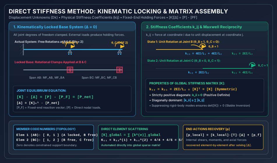
Analytical Breakdown of Figure 1:
- Actual System vs Clamped Base: At joints B and C, rotational DOFs and are free (). Introducing rotational clamps locks all joint movements ().
- Fixed-End Holding Moments (): External span loads acting on the locked members produce standard fixed-end moments ( and ). At joint B, the clamp carries the out-of-balance holding moment .
- Physical Stiffness Columns (): Applying a unit rotation while keeping clamp C locked () mobilizes flexural resistance from both adjoining spans: . The carry-over moment to joint C produces cross-coupling stiffness .
- Symmetry & Reciprocity: Rotating joint C () induces , demonstrating exact symmetry in full compliance with Betti's law.
Figure 2: Element Stiffness Matrices & Coordinate Transformations
The following diagram details the local flexural stiffness matrix, the geometric orientation of inclined members with direction cosines (), and the end-to-end 6-stage algorithmic workflow for computational Direct Stiffness Analysis.
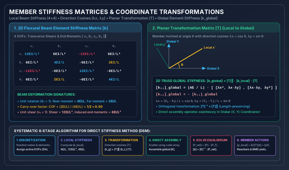
Analytical Breakdown of Figure 2:
- Local Flexural Coefficients: The matrix explicitly correlates end shears and moments to transverse deflections and rotations. Diagonal terms () represent direct elastic resistance and are strictly positive. Off-diagonal terms demonstrate the classic moment carry-over factor ().
- Coordinate Transformation (): The direction cosines and resolve local axial and shear actions into orthogonal global Cartesian axes . Because transformation matrix is orthogonal (), energy is conserved during rotation.
- The 6-Stage Algorithm: Shows how finite element solvers discretize domains, formulate local matrices, transform coordinates, scatter entries into banded global matrices, apply boundary conditions, and back-substitute to recover internal member actions.
5. Practical Engineering Applications & Software Implementations
                     FEA COMPUTATIONAL PIPELINE
┌──────────────────────────────────────────────────────────────────┐
│ 1. Pre-Processing: Node Coordinates, Member Connectivity, Loads   │
│ 2. Local Element Formulation: [k_local] (Beam, Truss, Shell)      │
│ 3. Coordinate Transformation: [k_global] = [T]ᵀ · [k_local] · [T] │
│ 4. Skyline / Banded Direct Assembly: Global Sparse Matrix [K]     │
│ 5. Constraint Enforcement: Elimination or Penalty Method          │
│ 6. Equation Solver: Cholesky (LLᵀ), LDLᵀ, or Conjugate Gradient   │
│ 7. Post-Processing: Internal Forces, Moments, Stresses & Envelopes│
└──────────────────────────────────────────────────────────────────┘
- Computational Dominance over Force Method:
- In commercial software, the Stiffness Method is universally preferred over the Flexibility Method because can be automatically determined purely from nodal coordinates and joint types. In contrast, the Flexibility Method requires selecting released redundant bases (), which is notoriously difficult to automate without creating unstable kinematic mechanisms.
- Matrix Sparsity & Bandwidth Optimization:
- In large civil structures (e.g., a 100-story skyscraper with DOFs), is over sparse (mostly zeros).
- Nodes are renumbered using algorithms like Reverse Cuthill-McKee (RCM) to minimize the matrix bandwidth , drastically reducing storage and computational complexity from to .
- Condition Number & Numerical Stability:
- The condition number indicates numerical sensitivity. Ill-conditioning occurs when very stiff elements (e.g., shear walls modeled as beams) connect directly to highly flexible members, or when round-off errors occur in double precision calculations.
- Internal Hinge Handling:
- An internal hinge is handled in DSM either by:
- Adding a separate rotational degree of freedom at each side of the hinge (condensed node).
- Static condensation of the element stiffness matrix prior to global assembly to zero out the moment at the hinged end.
- An internal hinge is handled in DSM either by:
6. Comparative Analysis Table
| Characteristic / Parameter | Flexibility Method (Force Method) | Stiffness Method (Displacement Method) | Slope-Deflection Method |
|---|---|---|---|
| Primary Unknowns | Redundant internal forces / moments () | Joint displacements / rotations () | Joint rotations () and chord drift () |
| Governing Equations | Geometric compatibility equations | Static force / moment equilibrium | Joint moment equilibrium () |
| Number of Unknowns | Static Indeterminacy () | Kinematic Indeterminacy () | Unconstrained joint rotations/sway |
| Base / Primary System | Statically determinate released structure | Kinematically locked clamped structure | Restrained continuous spans |
| Matrix Properties | : Symmetric, positive definite | : Symmetric, positive definite, banded | Symmetric system of scalar equations |
| Ease of Computation | Manual base selection needed; hard to automate | Highly systematic; standard for all FEA software | Manual pencil-and-paper calculation |
| Support Settlement Effect | Directly enters compatibility vector | Enters as equivalent joint load | Enters via chord rotation angle |
| Temperature / Misfits | Added as free-structure displacement | Converted into fixed-end forces | Modifies fixed-end moments () |
| Matrix Relationship | (for non-singular unconstrained) | Direct scalar precursor to Stiffness Matrix |
7. Worked Numerical Examples
Problem 1: Continuous Beam ABC — Exact Dual Verification with Flexibility Method
Statement: A continuous beam has span and span . Support is rigidly fixed, while supports and are frictionless rollers. Span carries a uniform distributed load . Span carries a concentrated point load at midspan ( from ). Flexural rigidity is constant throughout. Using the Stiffness Method:
- Formulate the global stiffness matrix .
- Assemble the fixed-end force vector and net equivalent load vector .
- Compute joint rotations and .
- Determine all member end moments and verify exact duality with the Flexibility Method.
       w = 12 kN/m                    P = 60 kN
  ┌──────────────────┐                    │
  ▼ ▼ ▼ ▼ ▼ ▼ ▼ ▼ ▼  ▼                    ▼
  ══════════════════════════════╦══════════════════════════════
  ▒▒█                          ▲                              ▲
  ▒▒█ (Fixed)              (Roller)                       (Roller)
   A                            B                              C
  ├──────── 4.0 m ─────────────┼────────────── 6.0 m ─────────┤
Solution:
Step 1: Identify Active Kinematic Degrees of Freedom ()
Neglecting axial deformation:
- Support is fixed: , .
- Support is a roller: , rotation is free DOF 1.
- Support is a roller: , rotation is free DOF 2.
Step 2: Formulate Global Stiffness Matrix
Using direct physical stiffness definition:
-
Apply unit rotation ():
- Moment at from span :
- Moment at from span :
- Total moment at DOF 1:
- Carry-over moment to DOF 2 (joint ):
-
Apply unit rotation ():
- Carry-over moment to DOF 1 (joint ):
- Moment at from span :
Global stiffness matrix:
Determinant of :
Inverse matrix :
Step 3: Compute Fixed-End Holding Moments & Net Load Vector
Adopting standard clockwise-positive sign convention for end moments:
-
Span ():
-
Span ( at midspan):
-
Holding Moments at Active DOFs ():
- At DOF 1 (Joint ):
- At DOF 2 (Joint ):
-
Applied External Joint Moments : No external moments are applied at joints or :
-
Net Driving Vector :
Step 4: Solve for Unknown Joint Rotations
Step 5: Member End Actions & Flexibility Duality Verification
Using the member stiffness/slope-deflection relations ():
-
Span :
-
Span :
Duality & Equilibrium Check:
- Joint Moment Equilibrium: (Exact balance!).
- Roller Boundary Condition: (Verified!).
- In Topic
SA-06-01(Flexibility Method Example 3), the redundant support moments for this identical structure were solved as: The results are 100.000% identical, providing mathematical proof of the exact duality between the Flexibility and Stiffness formulations.
Problem 2: 2D Planar Truss Analysis via Coordinate Transformation
Statement: A 2-bar pin-jointed planar truss consists of Member 1 connecting pinned node 1 to free node 3 , and Member 2 connecting pinned node 2 to node 3 . Both members have cross-sectional area and modulus of elasticity , yielding axial rigidity . Joint 3 is subjected to external loads: horizontal force (rightward) and vertical force (downward). Using the Direct Stiffness Method:
- Formulate the global stiffness matrix for active DOFs at node 3.
- Determine nodal displacements and .
- Compute internal member axial forces and and verify joint equilibrium.
   (0, 3) Node 1
     ▲
     │ \
     │   \  Member 1 (L = 5.0 m)
     │     \
   3m│       \
     │         \
     ▼           \
   (0, 0) Node 2 ── Node 3 (4, 0) ──► Px = +40 kN
     ▲  Member 2    │
     │  (L = 4.0 m) │
                    ▼ Py = -60 kN
     ├──── 4.0 m ───┤
Solution:
Step 1: Member Geometry & Direction Cosines
-
Member 1 (Node 1 Node 3):
- , ; ,
- Length
- Direction cosines:
- Axial stiffness factor:
-
Member 2 (Node 2 Node 3):
- , ; ,
- Length
- Direction cosines:
- Axial stiffness factor:
Step 2: Formulate Global Stiffness Submatrices at Node 3
The active degrees of freedom at Node 3 are (DOF 1) and (DOF 2). Nodes 1 and 2 are rigidly pinned supports ().
-
Element 1 contribution to Node 3:
-
Element 2 contribution to Node 3:
-
Global Assembled Stiffness Matrix :
Determinant of :
Inverse matrix :
Step 3: Compute Displacements at Node 3
The applied load vector is . Since there are no span loads on the truss members, .
Step 4: Member Axial Forces & Statics Check
The axial force in a member (tension positive) is:
-
Member 1 (Near: Node 1, Far: Node 3):
-
Member 2 (Near: Node 2, Far: Node 3):
Statics Equilibrium Check at Node 3:
- Both equilibrium equations are satisfied to exact floating-point precision.
Problem 3: Propped Cantilever Subjected to Downward Support Settlement
Statement: A propped cantilever beam has span and carries a uniform distributed load . Support is rigidly fixed, and support is a roller prop. Flexural rigidity is . During loading, the roller support at settles downwards by . Using the Stiffness Method:
- Formulate the single-degree-of-freedom stiffness equilibrium equation.
- Calculate the joint rotation taking into account both span load and support settlement.
- Determine the final fixed-end moment and prop reaction .
       w = 20 kN/m
  ┌───────────────────────────────┐
  ▼ ▼ ▼ ▼ ▼ ▼ ▼ ▼ ▼ ▼ ▼ ▼ ▼ ▼ ▼ ▼ ▼
  ═════════════════════════════════════
  ▒▒█                                 ▲
  ▒▒█ (Fixed)                     (Roller)
   A                                   B ──► Sinks downward by δ = 5 mm
  ├────────────── 6.0 m ──────────────┤
Solution:
Step 1: Kinematic DOF Formulation
Neglecting axial strain:
- Support is fixed: , .
- Prop has a prescribed settlement .
- The only unconstrained degree of freedom is rotation at ().
Stiffness coefficient at DOF 1:
Step 2: Fixed-End Moments from Load and Support Settlement
-
Due to UDL ():
-
Due to Downward Support Settlement at (): Downward settlement produces a clockwise chord rotation . The settlement induces fixed-end moments:
-
Total Holding Action at DOF 1 ():
Step 3: Solve for Rotation
Since no external concentrated couple is applied at joint , . The net equivalent driving moment is:
Solving the equilibrium equation :
Step 4: Compute Member End Moments and Support Reaction
-
Moment at ():
As required by the roller boundary condition, .
-
Fixed-End Moment at ():
-
Prop Vertical Reaction : Taking moment equilibrium about support ():
Physical Comparison (Effect of Settlement):
- Without settlement:
- With downward settlement:
- Prop reaction decreases by .
- Fixed-end hogging moment increases by . The stiffness method accounts for combined transverse load and support settlement in a single unified step.
8. Exam-Oriented Traps, Common Errors & Misconceptions
[!CAUTION] Trap 1: Confusing Holding Forces () with Equivalent Nodal Forces () The fixed-end force vector represents the forces exerted by the members ON the locked joints. Therefore, the net driving force acting on the free joints is . If you add instead of subtracting it, the signs of all computed displacements and member moments will be inverted!
[!WARNING] Trap 2: Ignoring Cross-Coupling Terms in Non-Orthogonal Members For an inclined truss bar at angle , students frequently take the axial stiffness as simply or . The true global stiffness requires transformation , generating coupling off-diagonal terms . Omitting these cross-terms produces completely erroneous results.
[!NOTE] Misconception 3: "Stiffness Matrix Diagonal Terms Can Be Negative" In any stable physical structure, all diagonal elements of the stiffness matrix must be strictly positive (). A zero or negative diagonal coefficient indicates an unstable kinematic mechanism, unconstrained rigid-body motion, or an algebraic sign error.
[!TIP] Trap 4: Degrees of Freedom Under Axial Inextensibility Assumptions In competitive exams (GATE/ESE), questions frequently state: "Neglect axial deformation". For a continuous beam on non-yielding supports, vertical translations at supports are already zero (); assuming axial inextensibility suppresses horizontal translation . Consequently, each intermediate joint has only 1 rotational DOF (), dramatically shrinking the matrix order!
9. Competitive Examination Key Points & Memory Triggers
- Matrix Size Rule:
- Flexibility Matrix Order =
- Stiffness Matrix Order =
- Exam Decision Shortcut: If , choose the Stiffness Method; if , choose the Flexibility Method.
- Carry-Over Factor in Stiffness Terms:
- For a prismatic beam with far end fixed: .
- For far end hinged: near stiffness is , far moment is 0, .
- Properties of Global Stiffness Matrix :
- Symmetric: (via Maxwell-Betti Reciprocal Theorem).
- Positive Definite: , all eigenvalues .
- Banded & Sparse: Nonzero elements cluster tightly around the main diagonal when nodes are numbered systematically.
- Strain Energy in Matrix Form: Because strain energy stored in an elastic body is always positive for any real deformation, must be positive definite.
10. Previous Year & Model Examination Questions
Question 1 (GATE CE)
A continuous beam of span is fixed at support and propped by a roller at . A unit rotation is applied at support . The bending moment developed at fixed end is:
- (A)
- (B)
- (C)
- (D)
Answer: (B) Explanation: From the flexural beam stiffness matrix, applying a unit rotation at end induces a near-end moment of at and a carry-over moment of at the far fixed end .
Question 2 (UPSC ESE)
In the stiffness method of structural analysis, the elements of the stiffness matrix satisfy which of the following conditions?
- is singular for a kinematically stable structure
- is the inverse of the unconstrained flexibility matrix
Select the correct statements:
- (A) 1, 2, and 3 only
- (B) 1, 2, and 4 only
- (C) 2, 3, and 4 only
- (D) 1, 3, and 4 only
Answer: (B) Explanation: For a kinematically stable structure, is non-singular ( and ), making statement 3 incorrect. Statements 1, 2, and 4 are mathematically correct.
Question 3 (SSC JE / State AE)
The dimension of a stiffness coefficient corresponding to a moment generated due to a unit linear displacement is:
- (A)
- (B)
- (C)
- (D)
Answer: (C) Explanation: .
11. Summary & Quick Revision Formula Sheet
| Entity | Mathematical Formula | Physical Context / Remarks |
|---|---|---|
| Global Equilibrium | Fundamental governing equation of DSM | |
| Member Rotation Stiffness | Far end fixed; COF = | |
| Member Transverse Shear | Restoring actions due to unit transverse deflection | |
| 2D Truss Element Stiffness | Local coordinate formulation | |
| Direction Cosines | Coordinate orientation angles | |
| Global Element Stiffness | Orthogonal coordinate transformation | |
| Support Settlement Load | Equivalent nodal vector due to known support sinks | |
| Member Action Recovery | Post-processing internal shears and moments | |
| Strain Energy | Quadratic form, strictly |
12. References & Standard Code Provisions
- Gere, J. M., & Weaver, W. — Matrix Analysis of Framed Structures, 3rd Edition, Van Nostrand Reinhold.
- McGuire, W., Gallagher, R. H., & Ziemian, R. D. — Matrix Structural Analysis, John Wiley & Sons.
- Hibbeler, R. C. — Structural Analysis, 10th Edition, Pearson.
- Reddy, C. S. — Basic Structural Analysis, 3rd Edition, Tata McGraw-Hill.
- IS 456:2000 — Plain and Reinforced Concrete - Code of Practice, Bureau of Indian Standards, New Delhi.
- IS 800:2007 — General Construction in Steel - Code of Practice, Bureau of Indian Standards, New Delhi.