Müller-Breslau Principle for Indeterminate Structures
In this chapter (4 topics)
On this page
- 1. Module Header & Metadata Block
- 2. Theoretical Foundations & Physical Concepts
- 2.1 The Breakthrough of Heinrich Müller-Breslau (1886)
- 2.2 Determinate vs Indeterminate Structures: The Elastic Difference
- 3. Mathematical Derivations & Analytical Formulations
- 3.1 First-Principles Derivation via Betti's Reciprocal Theorem
- 3.2 Types of Constraints & Imposed Displacements
- 3.3 Quantitative Influence Lines for Classical Indeterminate Beams
- 4. Critical Conditions & Governing Theorems
- 4.1 The Alternating Span Loading Rule (Müller-Breslau Criterion)
- 5. Cross-Sectional & Engineering Schematics
- 5.1 Qualitative Müller-Breslau Influence Lines for Beams and Frames
- 5.2 Quantitative Influence Lines: Propped Cantilever and Two-Span Beam
- 6. Solved Numerical Examples
- Example 1: Quantitative Analysis of a Propped Cantilever Girder
- Example 2: Peak Hogging Moment in a Two-Span Continuous Bridge Deck
- Example 3: Alternating Span Loading Pattern for a 3-Span Viaduct
- 7. Engineering Design Applications & Field Practice
- 7.1 IRC:6 and IS:456 Envelope Pattern Loading
- 7.2 Experimental Verification: Beggs Deformeter & Spline Models
- 8. Comparative Analysis & Summary Matrix
- 8.1 Comparison of ILD Characteristics Across Structural Types
- 9. Common Misconceptions & Exam Pitfalls
- 10. Previous Years' Examination Analysis & Reference Questions
- 10.1 Typical Competitive Examination Questions
- 11. Practice Problems with Answer Keys
- Problem 1 (Propped Cantilever Reaction Ordinate)
- Problem 2 (Two-Span Continuous Beam Hogging Moment)
- Problem 3 (Alternating Span Loading Identification)
- 12. Comprehensive Subject & Examination Mapping
1. Module Header & Metadata Block
- Topic ID:
SA-04-04 - Module: Structural Analysis (Subject 03)
- Chapter: Chapter 04: Influence Line Diagrams & Moving Loads
- Title: Müller-Breslau Principle for Indeterminate Structures
- Target Examinations:
- GATE Civil Engineering (Structural Engineering)
- UPSC Engineering Services Examination (ESE/IES Paper-I)
- SSC JE Civil Engineering (Theory of Structures)
- State Public Service Commission Assistant Engineer (AE) & Junior Engineer (JE) Examinations
- Railway Recruitment Board Junior Engineer (RRB JE)
- Prerequisites:
- Topic
SA-02-02: Castigliano's Theorems, Betti's Law & Maxwell's Reciprocal Theorem - Topic
SA-03-01: Propped Cantilevers & Fixed Beams - Topic
SA-04-01: Influence Lines for Determinate Beams & Girders
- Topic
- Learning Objectives:
- State and rigorously prove the Müller-Breslau Principle using Betti's Reciprocal Theorem.
- Sketch accurate qualitative influence line diagrams for redundant reactions, support bending moments, midspan moments, and internal shear forces in continuous beams and rigid portal frames.
- Formulate and apply the Alternating Span Loading Rule to determine critical vehicular positions for maximum sagging and hogging moments in continuous bridge decks.
- Derive exact quantitative influence line equations for classical indeterminate structures, including propped cantilevers and two-span continuous beams.
- Calculate exact maximum internal forces and reactions under moving concentrated loads and uniformly distributed loads using influence line deflection integrals.
2. Theoretical Foundations & Physical Concepts
2.1 The Breakthrough of Heinrich Müller-Breslau (1886)
Prior to 1886, determining influence lines for statically indeterminate structures required setting up and solving tedious systems of simultaneous equilibrium and compatibility equations for every discrete position of a moving unit load.
German structural engineer Heinrich Müller-Breslau established a revolutionary kinematic theorem that connects influence lines directly to the deflected elastic shapes of structures:
[!IMPORTANT] The Müller-Breslau Principle: The influence line for any reaction or internal force (moment, shear, or axial force) of a linear elastic structure is, to some scale, the deflected shape of the structure obtained by:
- Removing the restraint corresponding to that force/reaction.
- Introducing a unit displacement (or unit rotation or unit relative slip) in the positive direction of the released force.
2.2 Determinate vs Indeterminate Structures: The Elastic Difference
The Müller-Breslau Principle is universally applicable to both statically determinate and indeterminate structures:
-
Statically Determinate Structures:
- Removing one restraint reduces the degree of static determinacy from to , transforming the structure into an unstable rigid-body mechanism (single degree of freedom).
- The members undergo rigid-body rotation without any bending strain ().
- Therefore, the influence line consists entirely of straight line segments.
-
Statically Indeterminate Structures:
- Removing one restraint from a structure with indeterminacy leaves a stable structure with degree of indeterminacy .
- Introducing a unit displacement induces internal bending moments, curvature, and elastic flexural deformation ().
- Therefore, the influence line is a smooth, continuous curved line (cubic or higher-order polynomial deflection curve).
3. Mathematical Derivations & Analytical Formulations
3.1 First-Principles Derivation via Betti's Reciprocal Theorem
Consider a linearly elastic, statically indeterminate structure (such as a continuous beam or propped cantilever) supported at several points.
Let:
- A unit vertical downward load act at an arbitrary location along the span.
- be the redundant reaction or internal force component whose influence line is sought (e.g., redundant reaction , support moment , or shear ).
We define two distinct load-displacement states:
  STATE 1: Actual Structure Under Moving Unit Load
                 P = 1 (at x)
                 v
     A o=========+===========B===========o C
             (Reaction / Internal Force X_i develops)

  STATE 2: Auxiliary Structure (Restraint Released, Unit Displacement Applied)
                 F_i causes Δ_i = 1.0
                 ^
     A o=========+===========o===========o C
             Deflected profile = δ(x)
State 1: Actual Structure
- A unit vertical load acts downward at coordinate .
- Under this loading, the structure develops the redundant force .
- Because the actual boundary condition or structural continuity is intact, the displacement at coordinate is zero: .
State 2: Auxiliary Released Structure
- The restraint corresponding to is removed.
- An auxiliary force is applied at coordinate such that it produces a unit displacement in the direction of :
- Under this unit displacement, the beam deflects into an elastic curve at all points . The vertical deflection at coordinate is denoted as (measured positive downward, in the direction of ).
Application of Betti's Law of Reciprocal Work
Betti's Law states that for any linear elastic system, the virtual work done by the forces of State 1 acting through the displacements of State 2 equals the virtual work done by the forces of State 2 acting through the displacements of State 1:
Evaluating the virtual work terms:
-
LHS (Forces of State 1 through Displacements of State 2):
- The force (acting downward at ) moves through vertical displacement (downward):
- The reactive force acts against the imposed displacement :
- Support reactions at unreleased supports move through zero displacement.
-
RHS (Forces of State 2 through Displacements of State 1):
- In State 2, the only external force applied is at coordinate .
- In State 1, the displacement at coordinate is identically zero () because the actual structure has an unyielding constraint at that coordinate!
Equating LHS to RHS:
[!IMPORTANT] Mathematical Equation of the Müller-Breslau Principle: For any general non-unit imposed displacement :
The influence line ordinate at any position is identically equal to the deflection of the released structure subjected to a unit displacement at the location and in the direction of the redundant .
3.2 Types of Constraints & Imposed Displacements
| Target Quantity | Released Constraint | Imposed Unit Displacement | Deflection Condition | Resulting ILD |
|---|---|---|---|---|
| Support Reaction () | Remove support constraint (roller or pin) | Apply vertical displacement upward | Slope continuity preserved at | Continuous cubic curve |
| Support Moment () | Insert internal hinge at support | Apply unit relative rotation | Discontinuous slope (kink ) at | Downward cusped curve (hogging) |
| Span Moment () | Insert internal hinge at section | Apply unit relative rotation | Discontinuous slope (kink ) at | Upward cusped curve (sagging) |
| Transverse Shear () | Insert sliding shear release (guide) at | Apply unit relative vertical slip | Tangents remain strictly parallel () | Vertical step jump |
3.3 Quantitative Influence Lines for Classical Indeterminate Beams
3.3.1 Propped Cantilever Beam (Span , Fixed at , Roller Prop at )
Consider a propped cantilever beam of span and flexural rigidity .
     Fixed A                         Roller B
      |================================o
     x=0            Span L            x=L
(a) ILD for Prop Reaction
- Release: Remove roller support at . The structure becomes a cantilever fixed at .
- Impose Unit Load at : Apply unit upward load at tip .
- Deflection Equation: Measuring from the fixed support (): The bending moment at distance from is . Using the elastic curve differential equation :
- Tip Deflection at ():
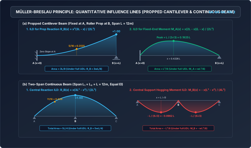
- Influence Line Equation for :
- Boundary Values:
- At fixed support ():
- At midspan ():
- At prop ():
- Area under the ILD: Under a full span UDL of intensity , the prop reaction is .
(b) ILD for Fixed-End Moment
- By Static Equilibrium: When a unit load is at position from fixed end :
- Stationary / Peak Point:
- Peak Moment Magnitude: Substituting :
- Area under the ILD: Under full UDL : .
3.3.2 Two-Span Continuous Beam (Span , Constant )
Consider a continuous beam over three simple supports , , and , with equal spans .
     Pin A            Roller B           Roller C
      o==================o==================o
     x=0     Span L     x=L     Span L     x=2L
(a) ILD for Central Support Reaction
- Release: Remove support . The structure becomes a simply supported beam of span .
- Apply Unit Load at : Apply unit upward load at center .
- Midspan Deflection:
- Deflection Curve for :
- Influence Line Equation for :
- Key Ordinates:
- At support ():
- At midspan of span ():
- At central support ():
- Total Area over both spans (): Under full UDL on both spans: .
(b) ILD for Central Support Hogging Moment
By Clapeyron's Three-Moment Equation, when a unit downward load sits at distance from ():
Since supports and are simply supported, :
- Peak Hogging Moment Location:
- Peak Hogging Moment Magnitude:
- Area under the ILD over One Span:
- Total Moment under Full Span UDL (Both Spans Loaded):
4. Critical Conditions & Governing Theorems
4.1 The Alternating Span Loading Rule (Müller-Breslau Criterion)
To maximize any given internal force or moment in a multi-span continuous beam:
-
Maximum Positive (Sagging) Moment in Span :
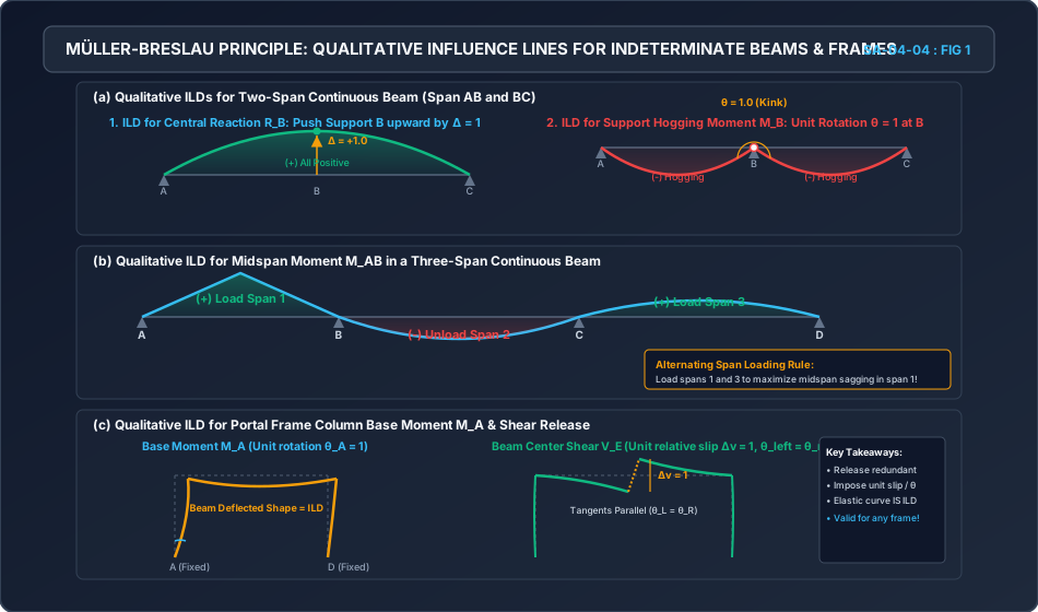
- Draw the qualitative ILD (unit upward kink at the section).
- The ILD has positive lobes in span , span , span , etc. (alternate spans).
- The ILD has negative lobes in adjacent spans , span , etc.
- Loading Rule: Apply live load to span and all alternate spans (). Leave adjacent spans completely unloaded!
-
Maximum Negative (Hogging) Moment at Interior Support :
- Draw the qualitative ILD (unit rotation at support ).
- Both spans meeting at support (span and span ) have large negative downward lobes.
- Alternate outer spans have smaller positive lobes.
- Loading Rule: Apply live load to both spans adjacent to support , and to every alternate span beyond!
  Midspan Sagging in Span 1:
     (+) Load Span 1       (-) Unload Span 2     (+) Load Span 3
    [=================]                         [=================]
   A o-----------------B-----------------------C-----------------o D

  Support Hogging at B:
     (-) Load Span 1       (-) Load Span 2       (+) Unload Span 3
    [=================]   [=================]
   A o-----------------B-----------------------C-----------------o D
5. Cross-Sectional & Engineering Schematics
5.1 Qualitative Müller-Breslau Influence Lines for Beams and Frames
The following schematic illustrates the qualitative deflected shape construction for reactions, moments, and shears in continuous beams and rigid portal frames:
5.2 Quantitative Influence Lines: Propped Cantilever and Two-Span Beam
The following engineering diagram provides the exact mathematical curves, critical station ordinates, and area integrals for propped cantilevers and continuous beams:
6. Solved Numerical Examples
Example 1: Quantitative Analysis of a Propped Cantilever Girder
Problem Statement: A steel propped cantilever beam has a clear span of and flexural rigidity . The left end is rigidly fixed, and the right end is supported on an unyielding roller prop. A moving load system consists of:
- A concentrated wheel load of .
- A uniformly distributed dead load of spanning the entire beam.
- A rolling live load UDL of of length .
Determine:
- The prop reaction and fixed-end moment when the point load is at midspan ().
- The position of point load to produce the absolute maximum fixed-end moment , and its magnitude.
- The total maximum prop reaction developed under the combined action of dead load, point load , and rolling UDL .
Solution:
Step 1: Reactions for Point Load at Midspan ()
Using the derived quantitative formulas with , :
- Prop Reaction ILD Ordinate:
- Fixed-End Moment ILD Ordinate:
Step 2: Absolute Maximum Fixed-End Moment under Point Load
From the mathematical derivation, maximum occurs when:
Peak ILD Ordinate:
Absolute Maximum Moment:
Step 3: Total Maximum Prop Reaction
- Dead Load Contribution (Full Span UDL):
- Point Load Contribution (): Maximum when placed directly over prop (, ):
- Live Load UDL Contribution (, length ):
To maximize , place the UDL adjacent to prop (from to ):
- At :
- At :
- Total Combined Maximum Prop Reaction:
Example 2: Peak Hogging Moment in a Two-Span Continuous Bridge Deck
Problem Statement: A two-span continuous reinforced concrete bridge girder has equal spans of (). A heavy trailer axle of weight traverses the bridge from left to right.
- Determine the exact longitudinal position of the axle from support to produce the maximum hogging bending moment at the central pier .
- Calculate the magnitude of this maximum hogging moment ().
- If a continuous live load train of crosses the bridge, calculate the maximum hogging moment developed at pier when both spans are fully covered.
Solution:
Step 1: Critical Position of Axle
The ILD equation for hogging moment at for load on span () is:
Peak hogging moment occurs at:
Step 2: Magnitude of Maximum Hogging Moment under Axle
Peak ILD Ordinate:
Maximum Hogging Moment:
Step 3: Moment under Full Span UDL ()
The area under the ILD for each span is:
For both spans fully loaded:
Verification via Clapeyron formula:
Example 3: Alternating Span Loading Pattern for a 3-Span Viaduct
Problem Statement: A three-span continuous prestressed concrete viaduct has equal spans of (). Dead load of the superstructure is . Design live load is . Using the Müller-Breslau Principle:
- Sketch the qualitative ILD for midspan moment in the central span ( from ).
- Identify which spans must be loaded with live load to generate:
- Maximum positive (sagging) bending moment at .
- Maximum negative (hogging) bending moment at .
- Sketch the qualitative ILD for support moment , and identify which spans must be loaded to maximize hogging at .
Solution:
Step 1: Qualitative ILD for Midspan of Center Span ()
- Insert an internal hinge at midspan of span .
- Impose unit relative upward rotation :
- Span arches upward into a positive (sagging) lobe.
- As the beam passes through support , it curves downward into span , creating a negative (hogging) lobe.
- As the beam passes through support , it curves downward into span , creating a negative (hogging) lobe.
         Span AB (-)            Span BC (+)            Span CD (-)
       (Negative Lobe)        (Positive Lobe)        (Negative Lobe)
   A o-----------------B---------o---------C-----------------o D
                                 E
Step 2: Critical Live Load Patterns for Midspan
- To Produce Maximum Positive (Sagging) Moment at :
- Dead Load: Placed on all three spans ().
- Live Load: Placed only on Span (the span containing the positive lobe). Spans and must remain unloaded by live load!
- To Produce Maximum Negative (Hogging) Moment at :
- Dead Load: Placed on all three spans.
- Live Load: Placed on Spans and (the spans containing negative lobes). Span must remain unloaded by live load!
Step 3: Critical Live Load Pattern for Support Pier ()
- Insert an internal hinge at support . Impose unit rotation :
- Beam sags downward into Span ().
- Beam sags downward into Span ().
- Beam arches upward into Span ().
- To Produce Maximum Hogging Moment at Support :
- Live load must be placed on Spans and (adjacent spans).
- Span must remain unloaded by live load!
7. Engineering Design Applications & Field Practice
7.1 IRC:6 and IS:456 Envelope Pattern Loading
In practical structural engineering for continuous reinforced concrete bridge decks and multi-storey building frames:
- Dead loads () are permanently present on all spans.
- Live loads () are movable. The structural engineer must evaluate three canonical load combinations:
- Case 1 (Full Load): on all spans (governs maximum support reactions and pier design).
- Case 2 (Alternate Spans Loaded): on odd spans, only on even spans (governs maximum midspan sagging moments).
- Case 3 (Adjacent Spans Loaded): on two adjacent spans, on remaining spans (governs maximum support hogging moments).
7.2 Experimental Verification: Beggs Deformeter & Spline Models
Before computer software (STAAD.Pro, SAP2000), engineers directly exploited the Müller-Breslau Principle experimentally:
- Beggs Deformeter (1922): A precision mechanical micro-gauge attached to celluloid or plexiglass scale models of indeterminate bridge portals.
- A calibrated micrometer imposed a precise mechanical displacement ( or ), and microscopes measured the deflected coordinates along the deck.
- The measured deflected shape yielded the exact quantitative influence lines for structures too complex for hand calculation!
8. Comparative Analysis & Summary Matrix
8.1 Comparison of ILD Characteristics Across Structural Types
| Attribute | Determinate Structures (Beams, Trusses, 3-Hinged Arches) | Indeterminate Structures (Propped Cantilevers, Continuous Beams, Portal Frames) |
|---|---|---|
| Influence Line Profile | Exclusively Straight Lines (Linear polygons) | Smooth Continuous Curves (Polynomial / Elastic flexural curves) |
| Physical Release Mechanism | Structure becomes a kinematic mechanism with zero flexural strain | Structure remains a stable elastic frame with flexural curvature |
| Effect of Member Stiffness () | Independent of (Pure equilibrium statics) | Dependent on Relative () |
| Effect of Support Sinking | No secondary stresses developed | Severe secondary moments and reaction redistribution |
| Mathematical Basis | Equations of Static Equilibrium () | Betti's Reciprocal Theorem & Müller-Breslau Principle |
9. Common Misconceptions & Exam Pitfalls
[!CAUTION] Trap 1: Assuming Müller-Breslau Only Applies to Indeterminate Structures
Students often answer that Müller-Breslau is invalid for determinate beams.
Reality: Müller-Breslau is universally valid for both. For determinate structures, removing a restraint creates a rigid mechanism, yielding straight lines. For indeterminate structures, it yields curved elastic lines.
[!WARNING] Trap 2: Drawing Angular Kinks in Support Reaction ILDs
When sketching the ILD for reaction of a continuous beam, students often draw a triangle with a sharp kink at support .
Reality: When support is pushed upward by , the beam is continuous across . The elastic curve has a smooth, continuous slope (), with no kink! Kinks occur only when an internal hinge is inserted (for bending moment ILDs).
[!WARNING] Trap 3: Forgetting the Parallel Tangent Rule for Shear ILDs
When introducing a shear release, students often rotate one side relative to the other.
Reality: A pure shear release transmits bending moment, which enforces . The tangents on either side of the vertical step jump must remain strictly parallel!
10. Previous Years' Examination Analysis & Reference Questions
10.1 Typical Competitive Examination Questions
Question 1 (GATE Civil Engineering)
The Müller-Breslau principle in structural analysis is used for:
- (A) Drawing the Influence Line Diagram for any force quantity
- (B) Writing the virtual work equation
- (C) Developing the flexibility matrix
- (D) Establishing dynamic equilibrium Solution: Option (A).
Question 2 (UPSC ESE / IES)
The influence line for bending moment at the fixed support of a propped cantilever of span reaches its maximum value when the load is placed at a distance from the fixed support equal to:
- (A)
- (B)
- (C)
- (D) Solution: Option (C) ().
Question 3 (SSC JE / State AE)
To obtain the influence line for the shear force at a cross-section of an indeterminate beam using the Müller-Breslau principle, the release introduced at that cross-section is:
- (A) An internal hinge
- (B) A guided roller permitting only vertical relative translation without rotation
- (C) Complete removal of the section
- (D) A propped support Solution: Option (B).
11. Practice Problems with Answer Keys
Problem 1 (Propped Cantilever Reaction Ordinate)
A propped cantilever of span is propped at . Calculate the ordinate of the influence line for prop reaction at a distance of from the fixed support .
Answer Key:
Problem 2 (Two-Span Continuous Beam Hogging Moment)
A two-span continuous beam has equal spans of . Calculate the maximum hogging moment developed at the interior pier when a single concentrated wheel load of rolls across the beam.
Answer Key:
- Peak ILD ordinate: .
- .
Problem 3 (Alternating Span Loading Identification)
A 4-span continuous bridge deck () carries moving traffic. To maximize the sagging moment at midspan of span , specify which spans must be loaded with live load.
Answer Key:
- By the alternating span rule, load Span and Span .
- Leave Spans and unloaded.
12. Comprehensive Subject & Examination Mapping
| Competitive Examination | Relevant Section / Paper | Expected Weightage | Typical Question Style |
|---|---|---|---|
| GATE CE | Structural Engineering (Analysis) | Multiple Choice / NAT questions on critical load location (, ), quantitative prop reaction, or qualitative deflected shape identification. | |
| UPSC ESE | Paper-I (Structural Analysis) | Conventional proof of Müller-Breslau from Betti's Law, qualitative sketching for complex frames, and quantitative integration under UDL. | |
| SSC JE | Theory of Structures | Conceptual questions on straight vs curved ILDs, type of release for shear/moment, and alternating span loading rules. | |
| State AE / JE | Civil Engineering Paper-I | Maximum hogging moment location in continuous beams, midspan ordinate for propped cantilever (), and frame qualitative sketches. | |
| RRB JE | Structural Mechanics | Definition of Müller-Breslau principle and identification of qualitative influence line shapes. |