Moment Distribution Method (Hardy Cross Method)
In this chapter (4 topics)
On this page
- 1. Introduction & Historical Significance
- 2. Mathematical Foundation & Fundamental Definitions
- 2.1 Sign Convention
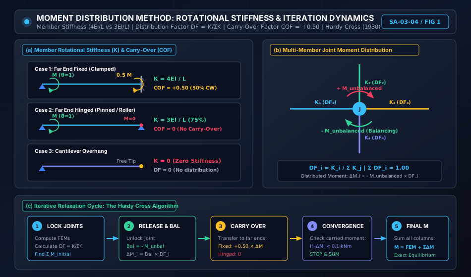
- 2.2 Member Rotational Stiffness (K)
- 2.3 Relative Stiffness (k)
- 2.4 Distribution Factor (DF)
- 2.5 Carry-Over Factor (COF)
- 3. Engineering Diagrams & Visual Explanations
- 3.1 Stiffness Profiles & Iteration Cycle
- 3.2 Portal Frame Sway Analysis Framework
- 4. Special Structural Considerations in Moment Distribution
- 4.1 Treatment of Cantilever Overhangs
- 4.2 Far End Hinged Shortcut (Modified Stiffness)
- 4.3 Support Sinking (Differential Settlement)
- 5. Side Sway Analysis of Portal Frames (Two-Stage Superposition)
- Stage 1: Non-Sway Analysis (Artificial Restraint)
- Stage 2: Arbitrary Sway Analysis
- Stage 3: Superposition with Sway Correction Factor k
- 6. Step-by-Step Analytical Algorithm
- 7. Solved Numerical Examples
- Example 1: Continuous Beam with Cantilever Overhang and Pinned Far End
- Example 2: Continuous Beam Subjected to Support Sinking
- Example 3: Side Sway Analysis of Portal Frame via Two-Stage Superposition
- 8. Practical Applications & Design Implications
- 9. Comparative Matrix: Classical Indeterminate Methods
- 10. Common Misconceptions & Exam Traps
- 1. Carrying Over Moments to a Pinned Support
- 2. The Modified Stiffness Trap
- 3. Forgetting the Balancing Moment Sign
- 11. Practice Problems
- Problem 1 (GATE CE Standard)
- Problem 2 (UPSC ESE Conventional Standard)
- 12. Quick Revision Formula Summary
1. Introduction & Historical Significance
The Moment Distribution Method, developed by Professor Hardy Cross and published in the May 1930 proceedings of the American Society of Civil Engineers (ASCE), is universally regarded as one of the greatest milestones in structural engineering history.
Before the advent of digital computers, analyzing continuous indeterminate frames using the Slope-Deflection Method or classical Force Methods required solving massive systems of simultaneous algebraic equations. In complex multi-story building frames, solving dozens or hundreds of coupled equations by hand was practically impossible.
Hardy Cross conceived an elegant, physically intuitive successive relaxation method:
- Instead of solving simultaneous equations, joints are artificially "locked" against rotation.
- Joints are then unlocked (released) one by one in an iterative cycle: unbalanced joint moments are distributed among meeting members in proportion to their rotational stiffnesses, and half of the distributed moment is "carried over" to the opposite ends.
- As the unbalanced increments diminish exponentially, the process converges rapidly to the exact theoretical solution.
Mathematical Classification:
┌────────────────────────────────────────────────────────────────────────┐
│ The Moment Distribution Method is a displacement method that performs │
│ successive Gauss-Seidel relaxation on the underlying Slope-Deflection  │
│ equilibrium equations without ever forming an explicit matrix!         │
└────────────────────────────────────────────────────────────────────────┘
2. Mathematical Foundation & Fundamental Definitions
The entire method rests on four fundamental concepts: Fixed-End Moments, Rotational Stiffness, Distribution Factor, and Carry-Over Factor.
2.1 Sign Convention
In accordance with classical displacement method standards:
- Clockwise member end moments acting on the joint or member end are taken as POSITIVE (+).
- Anticlockwise member end moments are taken as NEGATIVE (-).
2.2 Member Rotational Stiffness ()
Rotational Stiffness () is defined as the bending moment required to produce a unit rotation () at the near end of a member while maintaining the boundary condition at the far end:
Near End A (Rotated by θ = 1)                 Far End B
       (↻) M = K ────────────────────────────── [Support Condition]
Case 1: Far End Clamped / Fixed
When the far end is rigid and locked against rotation ():
where is Young's modulus, is the second moment of area, and is the member length.
Case 2: Far End Hinged / Pinned / Roller
When the far end is free to rotate without moment restraint ():
The rotational stiffness is reduced by exactly because the far end hinge offers no rotational restraint.
Case 3: Far End Guided Roller (Shear-Free, Slope-Restrained)
When the far end cannot rotate but can translate transversely:
Case 4: Cantilever Overhang
An overhanging span has a completely free end. It offers zero rotational restraint to the joint:
2.3 Relative Stiffness ()
When all members of a structure share the same modulus of elasticity ():
- Far end fixed:
- Far end hinged:
- Overhang:
2.4 Distribution Factor ()
When a rigid monolithic joint connecting members is subjected to an unbalanced moment , all meeting member ends rotate through the exact same joint rotation angle .
Because the moment developed in each member is , the total balancing moment is:
Dividing member moment by total joint moment yields the Distribution Factor ():
Axiom of Joint Distribution:
At every joint in a structure, the sum of distribution factors of all framing members must equal unity:
2.5 Carry-Over Factor ()
The Carry-Over Factor () is the ratio of the bending moment induced at the far end to the balancing moment applied at the near end:
- Far End Fixed: (The carried-over moment has the same algebraic sign / clockwise sense as the distributed moment).
- Far End Hinged / Roller: (A simple hinge cannot sustain or carry over moment).
3. Engineering Diagrams & Visual Explanations
3.1 Stiffness Profiles & Iteration Cycle
The diagram below presents the member rotational stiffness states, the joint moment distribution mechanism, and the circular flow of the iterative Hardy Cross cycle.
3.2 Portal Frame Sway Analysis Framework
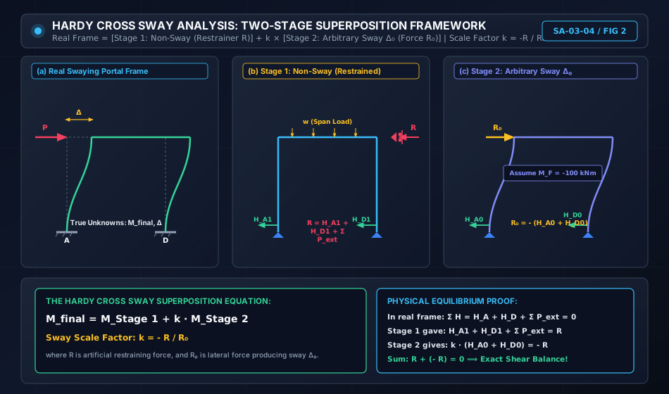
When portal frames are subjected to lateral loads or asymmetric conditions, side sway develops. The diagram below illustrates the classical Two-Stage Superposition method developed by Hardy Cross to solve frame sway.
4. Special Structural Considerations in Moment Distribution
4.1 Treatment of Cantilever Overhangs
When a continuous beam features an overhanging span extending beyond an exterior support:
- The cantilever moment is statically determinate: or .
- This determinate moment is placed directly in the initial moment row at the support.
- Because the cantilever has zero rotational stiffness (), its distribution factor is:
- Consequently, no balancing moment is ever distributed into the cantilever, and no moment is ever carried over from the cantilever.
4.2 Far End Hinged Shortcut (Modified Stiffness)
If an exterior support is a simple pin or roller (e.g., Support ):
- Standard Approach: Treat , carry over back and forth in every cycle, and observe the pinned end moment slowly oscillating to zero.
- The Modified Shortcut (Recommended):
- In Cycle 1, release and balance the exterior hinged support: .
- Carry over once to the interior adjacent support: .
- Lock the hinged support permanently.
- For all subsequent cycles, use the modified stiffness for that member:
4.3 Support Sinking (Differential Settlement)
If an interior support settles downward by :
- It induces initial Settlement Fixed-End Moments before the joints are unlocked:
- These settlement FEMs are added to the span load FEMs in the initial row, and standard distribution proceeds normally.
5. Side Sway Analysis of Portal Frames (Two-Stage Superposition)
In rigid portal frames, joint moment distribution enforces joint rotational equilibrium (), but cannot inherently satisfy global column horizontal shear equilibrium (). If lateral forces or asymmetries exist, the frame will experience lateral translation (sway ).
Hardy Cross solved this via a rigorous Two-Stage Superposition:
[Real Frame with Sway] = [Stage 1: Non-Sway Frame] + k × [Stage 2: Arbitrary Sway Frame]
Stage 1: Non-Sway Analysis (Artificial Restraint)
- Introduce an imaginary lateral roller support (restrainer) at the roof beam level to prevent sway ().
- Carry out standard moment distribution under the actual applied loads.
- From the resulting member end moments, calculate the horizontal column base shears:
- Calculate the artificial restraining force required to prevent sway:
- If , the frame is symmetric and non-swaying; Stage 1 gives the final moments!
- If , an artificial force is holding the frame. To neutralize it, the frame must be subjected to an equal and opposite lateral swaying force:
Stage 2: Arbitrary Sway Analysis
- Remove all applied transverse span loads.
- Impose an arbitrary lateral sway displacement to the right.
- Assume convenient arbitrary column sway fixed-end moments (typically for uniform columns):
- Distribute these sway FEMs through standard Hardy Cross cycles to obtain Stage 2 moments ().
- Calculate the resulting Stage 2 column shears and the lateral force that produces this arbitrary sway:
Stage 3: Superposition with Sway Correction Factor
To produce the exact required swaying force , the Stage 2 results must be scaled by:
The final member end moments throughout the frame are:
6. Step-by-Step Analytical Algorithm
[Step 1: Compute Member Stiffnesses & Distribution Factors]
  └─ Evaluate K = 4EI/L (fixed far end) or K = 3EI/L (hinged far end). K = 0 (cantilever).
  └─ At each joint: DF_i = K_i / Σ K_j. Verify Σ DF = 1.00.

[Step 2: Calculate Fixed-End Moments (FEMs)]
  └─ Compute standard FEMs (Clockwise +, Anticlockwise -).
  └─ Include settlement FEMs (-6EIΔ/L²) if applicable.

[Step 3: Setup the Distribution Table]
  └─ Columns: One column per member end (e.g., AB, BA, BC, CB, CD, DC).
  └─ Header: Enter Joint names and corresponding Distribution Factors.

[Step 4: Execute Initial Releases (Hinged Ends & Overhangs)]
  └─ Enter known determinate cantilever moments directly (DF = 0).
  └─ Release pinned ends once: Bal = - FEM_pin. Carry over +0.50 × Bal to interior support.
  └─ Modify interior member stiffness to 3EI/L and set COF = 0 for future cycles.

[Step 5: Perform Successive Distribution Cycles]
  └─ Balance: Compute unbalanced moment at joint: M_unbal = Σ M. Apply Bal = - M_unbal × DF.
  └─ Carry Over: Transfer 0.50 × Bal to opposite fixed ends.
  └─ Repeat until carried-over increments are negligible (< 0.10 kNm).

[Step 6: Algebraic Column Summation]
  └─ Sum all moments from the FEM row down to the last balancing row.
  └─ Verify joint equilibrium: Σ M_joint = 0.

[Step 7: Statics & Diagram Construction]
  └─ Determine span reactions from free-body equilibrium: R = R_0 ± (M_left + M_right)/L.
  └─ Construct final SFD and superposed BMD.
7. Solved Numerical Examples
Example 1: Continuous Beam with Cantilever Overhang and Pinned Far End
Problem Statement:
Analyze the continuous beam shown below using the Moment Distribution Method:
- Overhang : Length , carrying a concentrated load of at free tip .
- Span : Length , flexural rigidity . Load: Uniformly distributed load .
- Span : Length , flexural rigidity . Load: Central concentrated point load at midspan.
- Support is a roller with overhang. Support is a continuous roller. Support is a simple pin.
Determine all final member end moments and vertical support reactions.
       20 kN                  30 kN/m                         50 kN
         ↓            ┌───────────────────────┐                 ↓
  O ─────────── [▲] ──┴───────────────────────┴── [▲] ──────────┴────────── [▲]
     a = 2 m     A            L₁ = 6 m, 2EI        B         L₂ = 4 m, EI     C (Pin)
Solution:
Step 1: Overhang Determinate Moment
At support , the cantilever load produces an anticlockwise hogging moment on the beam:
For equilibrium of joint , the moment in member must balance the overhang:
Step 2: Member Rotational Stiffnesses & Distribution Factors at Joint
- Looking from to : Support is a simple roller support with known overhang moment (free to rotate) Far end hinged:
- Looking from to : Support is a simple pin Far end hinged:
- Total joint stiffness: .
- Distribution Factors:
Step 3: Fixed-End Moments (FEMs)
- Span ():
- Span ():
Step 4: Initial Releases & Modified Moments
-
Joint Release:
The moment at must be .
Balancing increment at .
Carry-over to .
Modified moment at : -
Joint Release (Pinned end ):
Balancing increment at .
Carry-over to .
Modified moment at :
Step 5: Moment Distribution at Joint (Single Exact Cycle)
Because both far ends and are now permanently released (hinged with and ), there are no carry-overs back to . The distribution converges in one single step!
- Unbalanced moment at :
- Balancing moment = .
- Distribution to :
- Distribution to :
Moment Distribution Table:
| Joint | O | A | B | C | ||
|---|---|---|---|---|---|---|
| Member | OA | AB | BA | BC | CB | |
| DF | - | - | 0.5714 | 0.4286 | - | |
| FEM | -40.00 | -90.00 | +90.00 | -25.00 | +25.00 | |
| Release A & C | - | +50.00 | - | - | -25.00 | |
| Carry-Over | - | - | +25.00 | -12.50 | - | |
| Modified Initial | -40.00 | +40.00 | +115.00 | -37.50 | 0.00 | |
| Balance B | - | - | -44.29 | -33.21 | - | |
| Final Moments | -40.00 | +40.00 | +70.71 | -70.71 | 0.00 |
Equilibrium Check at Joint B: .
Step 6: Support Reactions
- Support Reaction:
Taking moments about for the overhang and span : - Shear to right of in span :
- Span :
Taking moments about : - Total Reaction at Support :
Global Vertical Equilibrium Check:
Example 2: Continuous Beam Subjected to Support Sinking
Problem Statement:
A continuous beam consists of two equal spans .
- Flexural rigidity is constant.
- End is fixed, and end is pinned.
- Intermediate support sinks downward by .
- Neglect span loads to determine the pure settlement bending moments.
Solution:
Step 1: Settlement Fixed-End Moments (FEMs)
- Span : Support sinks relative to Clockwise chord rotation:
- Span : Support sinks relative to Anticlockwise chord rotation:
Step 2: Distribution Factors at Joint
- Far end is fixed: .
- Far end is pinned: .
- Total stiffness: .
Step 3: Initial Release of Pinned Support
- At support , . Balancing increment .
- Carry-over to .
- Modified initial moment at :
Step 4: Distribution at Joint
- Unbalanced moment at .
- Balancing moment .
- Carry-over to fixed end :
Moment Distribution Table:
| Joint | A | B | C | ||
|---|---|---|---|---|---|
| Member | AB | BA | BC | CB | |
| DF | - | 0.5714 | 0.4286 | - | |
| FEM (Sinking) | -100.00 | -100.00 | +100.00 | +100.00 | |
| Release C | - | - | - | -100.00 | |
| Carry-Over | - | - | -50.00 | - | |
| Modified Initial | -100.00 | -100.00 | +50.00 | 0.00 | |
| Balance B | - | +28.57 | +21.43 | - | |
| Carry-Over to A | +14.29 | - | - | - | |
| Final Moments | -85.71 | -71.43 | +71.43 | 0.00 |
Example 3: Side Sway Analysis of Portal Frame via Two-Stage Superposition
Problem Statement:
Analyze the portal frame shown below using the Hardy Cross Two-Stage Sway Superposition Method:
- Columns and have height and flexural rigidity . Bases and are fixed.
- Beam has span and flexural rigidity .
- A horizontal lateral load of acts at roof joint towards the right.
- No transverse span loads are present.
       P = 40 kN
       ───► B ─────────────────────────── C
            │        L = 5 m, EI          │
            │                             │
     h = 4m │ EI                       EI │ h = 4m
            │                             │
           [▲]                           [▲]
         Fixed A                       Fixed D
Solution:
Step 1: Distribution Factors
- Joint :
- By symmetry: .
Step 2: Stage 1 — Non-Sway Analysis
An artificial lateral support holds joint against sway ().
Because there are no span loads on , all Fixed-End Moments are zero:
- Stage 1 Column base shears: .
- Artificial Restraining Force required to hold the load:
- The force driving side sway is .
Step 3: Stage 2 — Arbitrary Sway Analysis
Apply an arbitrary sway displacement causing arbitrary column fixed-end moments:
Beam experiences no sway FEMs: .
Stage 2 Moment Distribution Table:
| Joint | A | B | C | D | |||
|---|---|---|---|---|---|---|---|
| Member | AB | BA | BC | CB | CD | DC | |
| DF | - | 0.5556 | 0.4444 | 0.4444 | 0.5556 | - | |
| Sway FEM | -100.00 | -100.00 | 0.00 | 0.00 | -100.00 | -100.00 | |
| Balance 1 | - | +55.56 | +44.44 | +44.44 | +55.56 | - | |
| Carry-Over 1 | +27.78 | - | +22.22 | +22.22 | - | +27.78 | |
| Balance 2 | - | -12.35 | -9.88 | -9.88 | -12.35 | - | |
| Carry-Over 2 | -6.17 | - | -4.94 | -4.94 | - | -6.17 | |
| Balance 3 | - | +2.74 | +2.20 | +2.20 | +2.74 | - | |
| Carry-Over 3 | +1.37 | - | +1.10 | +1.10 | - | +1.37 | |
| Balance 4 | - | -0.61 | -0.49 | -0.49 | -0.61 | - | |
| Stage 2 Sum | -85.29 | -70.59 | +70.59 | +70.59 | -70.59 | -85.29 |
Equilibrium Check: Joint : . Joint : .
Step 4: Arbitrary Sway Resistance
Column base shears produced by the Stage 2 moments:
The total lateral shear force producing this arbitrary sway is:
Step 5: Sway Correction Factor and Final Moments
Final moments: :
Step 6: Final Global Shear Equilibrium Verification
8. Practical Applications & Design Implications
- Pre-Computer Dominance in Structural Offices: From 1930 to 1980, almost every high-rise frame, continuous bridge, and industrial plant in India and worldwide was engineered using Hardy Cross tables.
- Rapid Field Checking of Software Output: Structural engineers frequently use a 2-cycle Hardy Cross calculation to verify software output (ETABS/STAAD) at critical transfer girder joints.
- Physical Insight into Structural Stiffness: Unlike finite element black-boxes, moment distribution visually demonstrates how stiffness attracts load: doubling a column's moment of inertia draws double the bending moment from the connecting floor girders.
9. Comparative Matrix: Classical Indeterminate Methods
| Feature | Moment Distribution Method | Slope-Deflection Method | Three-Moment Theorem | Direct Stiffness Matrix |
|---|---|---|---|---|
| Method Family | Displacement (Iterative) | Displacement (Closed-Form) | Force (Compatibility) | Displacement (Matrix) |
| Solving Engine | Successive numerical relaxation | Simultaneous linear equations | Tridiagonal recurrence | Inversion / Cholesky decomposition |
| Hand Calculation Suitability | Exceptional (No equations) | Tedious for | Fast for beams only | Unfeasible for hand calculation |
| Sway Treatment | Two-stage superposition | Incorporated in shear equation | Inapplicable to frames | Direct degrees of freedom |
| Convergence | Monotonic, geometric decay | Exact in one step | Exact in one step | Exact in one step |
10. Common Misconceptions & Exam Traps
[!WARNING]
1. Carrying Over Moments to a Pinned Support
Trap: Applying the carry-over factor to a far end that is a simple hinge.
Reality: A simple pin or roller support cannot resist bending moment (). Therefore, the Carry-Over Factor to a hinge is ALWAYS ZERO ()!
[!WARNING]
2. The Modified Stiffness Trap
Trap: Using for a hinged span from the very beginning without accounting for the pinned end's initial FEM.
Reality: If you use , you MUST first release the pinned end in Cycle 1, carry over to the interior joint, and only THEN use for subsequent balancing!
[!WARNING]
3. Forgetting the Balancing Moment Sign
Trap: Distributing .
Reality: To restore equilibrium, the balancing moment must oppose the unbalanced moment. The distributed moment is always:
11. Practice Problems
Problem 1 (GATE CE Standard)
A three-span continuous beam of uniform flexural rigidity has equal spans . Supports and are fixed; and are continuous rollers. If an external clockwise couple of is applied directly at joint , determine the final moment carried over to fixed support using the Moment Distribution Method.
Answer:
.
After iterative distribution through joints and : .
Moment carried over to : .
Problem 2 (UPSC ESE Conventional Standard)
A single-bay portal frame with fixed bases at and has columns () and roof beam (). A vertical point load of acts at midspan of .
Using the Moment Distribution Method, state whether the frame experiences side sway, compute the non-sway distribution, and find all final member end moments.
Answer:
Because the frame geometry, member properties, and loading are completely symmetric about the centerline, the artificial restraining force . The frame does NOT experience side sway!
, , , , , .