Stress-Strain Curves & IS 456 Parabolic-Rectangular Stress Block
In this chapter (3 topics)
On this page
- 1. Introduction & Conceptual Foundations
- 2. Assumptions of Limit State of Collapse in Flexure (IS 456:2000 Clause 38.1)
- 3. Mathematical Derivation of the Parabolic-Rectangular Stress Block
- 3.1 Geometry of the Strain Profile
- 3.2 Total Compressive Force (C)
- 3.3 Line of Action / Centroid of Compressive Force (bary)
- 3.4 Lever Arm (z) & Internal Resisting Moment (Mu)
- 4. Limiting Depth of Neutral Axis (xu,max / d)
- Limiting Values for Standard Steel Grades (IS 456:2000 Clause 38.1 Note)
- 5. Limiting Moment of Resistance (Mu,lim) & Steel Percentage (pt,lim)
- 5.1 Limiting Moment of Resistance (Mu,lim)
- 5.2 Limiting Tension Steel Percentage (pt,lim)
- 6. Constitutive Stress-Strain Behavior of Concrete
- 6.1 Compressive Behavior (IS 456 Figure 21)
- 6.2 Tensile Behavior & Modulus of Rupture
- 6.3 Modulus of Elasticity of Concrete
- 7. Constitutive Stress-Strain Behavior of Reinforcing Steel
- 7.1 Mild Steel (Fe 250) — Bilinear Model (IS 456 Figure 22)
- 7.2 High-Strength Deformed Bars (Fe 415, Fe 500) — Non-Linear Model (IS 456 Figure 23)
- 8. Worked Numerical Examples
- Problem 1: Integration & Verification of Concrete Stress Block Components
- Problem 2: Limiting Design Parameters Across Steel Grades
- Problem 3: Modulus of Rupture & Long-Term Creep Elasticity
- 9. Common Misconceptions & Exam Pitfalls
- 10. Comparative Summary & Master Formula Sheet
- Master Stress Block Parameters (IS 456:2000 Clause 38.1)
- 11. Practice Questions & Competitive Examination Problems
- Question 1 (GATE CE — 1 Mark)
- Question 2 (UPSC ESE — Objective)
- Question 3 (SSC JE — Technical)
- Question 4 (State AE — Analytical)
- Question 5 (GATE CE — 2 Marks)
- Question 6 (UPSC ESE — Conventional)
- 12. References & Code Standards
1. Introduction & Conceptual Foundations
In reinforced concrete design by the Limit State Method (LSM), the flexural capacity of a beam or slab is determined by the non-linear behavior of concrete in compression coupled with the yielding of tension reinforcement. While classical elastic theory (WSM) assumed linear triangular stress distributions based on Hooke's law, real concrete subjected to ultimate bending strains exhibits marked non-linear plasticity, micro-cracking, and strain softening.
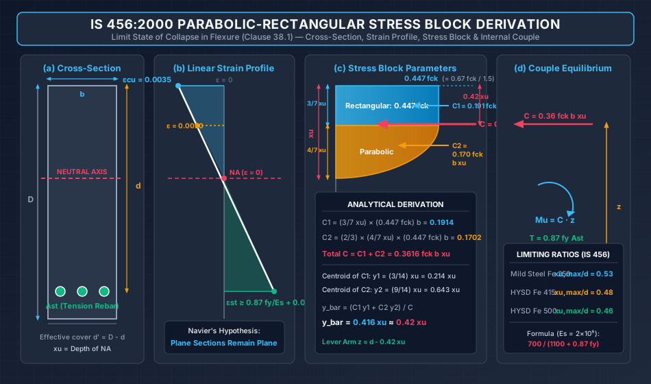
To accurately predict the ultimate flexural resistance () without performing tedious point-by-point numerical integration across the cross-section, IS 456:2000 Clause 38.1 idealizes the concrete compressive stress profile into a standardized Parabolic-Rectangular Stress Block.
This master technical note provides the complete, rigorous mathematical derivation of the stress block parameters ( and ), establishes the limiting neutral axis depth ratios (), and details the constitutive relationships for both concrete and reinforcing steel.
+----------------------------------------------------------------------------------------------------+
|                                 THE LIMIT STATE FLEXURAL MECHANISM                                 |
+----------------------------------------------------------------------------------------------------+
|                                                                                                    |
|    CROSS-SECTION             LINEAR STRAIN (Navier)              IS 456 STRESS BLOCK               |
|      +-------+                      |                                 |---- 0.447 fck              |
|      |       |                      | eps_cu = 0.0035                 |======|  Rectangular        |
|      |       | xu                   |                                 |======|  (3/7 xu)           |
|  ----+-------+---- NA       --------+-------- NA (eps = 0)    --------+---\  |                     |
|      |   O   |                      |                                      ) |  Parabolic          |
|      |  Ast  |                      |                                     /  |  (4/7 xu)           |
|      +-------+                      | eps_st >= 0.87fy/Es + 0.002            |                     |
|                                                                              v T = 0.87 fy Ast     |
+----------------------------------------------------------------------------------------------------+
2. Assumptions of Limit State of Collapse in Flexure (IS 456:2000 Clause 38.1)
Design for the limit state of collapse in flexure rests upon six foundational assumptions codified in IS 456:2000 Clause 38.1:
-
Navier's Hypothesis (Plane Sections Remain Plane):
Plane sections normal to the structural axis remain plane after bending across the entire depth of the member. This guarantees that the longitudinal strain varies strictly linearly with distance from the neutral axis: -
Maximum Compressive Strain in Concrete ():
The maximum strain in concrete at the outermost extreme compression fiber at flexural failure is taken as , irrespective of the concrete grade (). -
Idealized Compressive Stress Block:
The relationship between the compressive stress distribution in concrete and the compressive strain may be assumed to be a rectangle, trapezoid, parabola, or any other shape that predicts ultimate strength in close agreement with experimental tests.
IS 456:2000 codifies an idealized shape that is parabolic up to a strain of , followed by a constant rectangular stress plateau up to the ultimate strain of . -
Tensile Strength of Concrete Ignored:
The tensile strength of concrete is completely neglected in flexural strength calculations. All tension is resisted solely by the tensile reinforcement (). -
Steel Design Stress-Strain Relationship:
The stresses in the reinforcement are derived from the representative stress-strain curve for the type of steel used, with the material partial safety factor applied directly to the characteristic yield or proof strength (). -
Minimum Tensile Strain in Reinforcement at Failure:
To ensure that flexural members exhibit ductile, warning-rich yielding before concrete crushing (under-reinforced behavior), the tensile strain in the tension reinforcement at failure must satisfy:where is the modulus of elasticity of steel.
3. Mathematical Derivation of the Parabolic-Rectangular Stress Block
Consider a rectangular beam cross-section of width and effective depth , with neutral axis at depth from the extreme compression fiber.
3.1 Geometry of the Strain Profile
Because the strain varies linearly from at the neutral axis to at the top compression fiber:
where is the depth measured downwards from the extreme top compression fiber ().
Let be the depth at which the compressive strain equals the transition strain :
Thus, the compression zone divides into two distinct geometric portions:
- Rectangular Zone: From to , where strain .
The stress is uniform and equal to the design compressive strength: - Parabolic Zone: From to (height ), where strain drops from to .
The stress varies quadratically from down to at the neutral axis.
Top Fiber (z = 0) --------+---------------------------------+  sigma = 0.4467 fck
                          |                                 |
                          |      RECTANGULAR BLOCK          |  Height = 3/7 xu
                          |                                 |
Transition (z = 3/7 xu) --+---------------------------------+  eps = 0.0020
                          |                                /
                          |      PARABOLIC BLOCK          /    Height = 4/7 xu
                          |                              /
Neutral Axis (z = xu) ----+-----------------------------+      eps = 0, sigma = 0
3.2 Total Compressive Force ()
The resultant compressive force is the sum of the forces developed in the rectangular and parabolic zones:
1. Rectangular Portion ():
2. Parabolic Portion ():
The area of a second-degree parabola having base and height is given by Archimedes' formula ():
3. Combined Resultant Force ():
IS 456:2000 rounds this value to two decimal places:
3.3 Line of Action / Centroid of Compressive Force ()
Let be the depth of the centroid of the combined stress block measured downwards from the extreme top compression fiber. Taking first moments of area about the top fiber ():
1. Centroid of Rectangular Portion ():
2. Centroid of Parabolic Portion ():
For a parabola with its vertex at the top () and base at the neutral axis (), the centroid is located at of the parabolic height from the vertex:
3. Combined Centroid ():
IS 456:2000 rounds this factor to :
3.4 Lever Arm () & Internal Resisting Moment ()
The internal lever arm separating the resultant compressive force and the tensile force is:
The internal moment of resistance evaluated from the concrete compression side is:
Evaluated from the tension reinforcement side:
4. Limiting Depth of Neutral Axis ()
In a balanced section at the limit state of collapse, the extreme concrete fiber reaches its ultimate compressive strain simultaneously as the tension reinforcement reaches its minimum codified design yield strain:
From the linear strain profile across the depth (Navier's hypothesis), by similar triangles:
   Extreme Concrete Fiber
          |-------- eps_cu = 0.0035
          |       /
          |      /
   xu,max |     /
          |    /
   NA ----+---/---- (eps = 0)
          |  /
 d-xu,max | /
          |/
          |-------- eps_st = 0.87 fy / Es + 0.002
   Tension Steel Level
Inverting and adding to both sides:
Inverting to solve for the Limiting Neutral Axis Depth Ratio ():
Substituting the standard elastic modulus of reinforcing steel :
Limiting Values for Standard Steel Grades (IS 456:2000 Clause 38.1 Note)
| Steel Grade | Yield Strength () | Minimum Yield Strain | Exact Calculated Ratio | IS 456 Codified Value |
|---|---|---|---|---|
| Fe 250 (Mild Steel) | ||||
| Fe 415 (HYSD / TMT) | ||||
| Fe 500 (TMT) | ||||
| Fe 550D (High Ductility) |
Critical Observation for Exams:
The limiting depth of neutral axis depends exclusively on the grade of steel (). It is completely independent of the grade of concrete (). As the yield strength of steel increases, decreases.
5. Limiting Moment of Resistance () & Steel Percentage ()
5.1 Limiting Moment of Resistance ()
When , the section develops its maximum possible flexural capacity without compressive steel:
Dividing by :
where is the dimensionless limiting moment factor.
Calculation of per Steel Grade:
-
For Fe 250 ():
-
For Fe 415 ():
-
For Fe 500 ():
5.2 Limiting Tension Steel Percentage ()
From internal axial equilibrium :
Expressing as a percentage of cross-sectional area :
| Concrete Grade | Fe 250 () | Fe 415 () | Fe 500 () |
|---|---|---|---|
| M20 | |||
| M25 | |||
| M30 |
6. Constitutive Stress-Strain Behavior of Concrete
6.1 Compressive Behavior (IS 456 Figure 21)
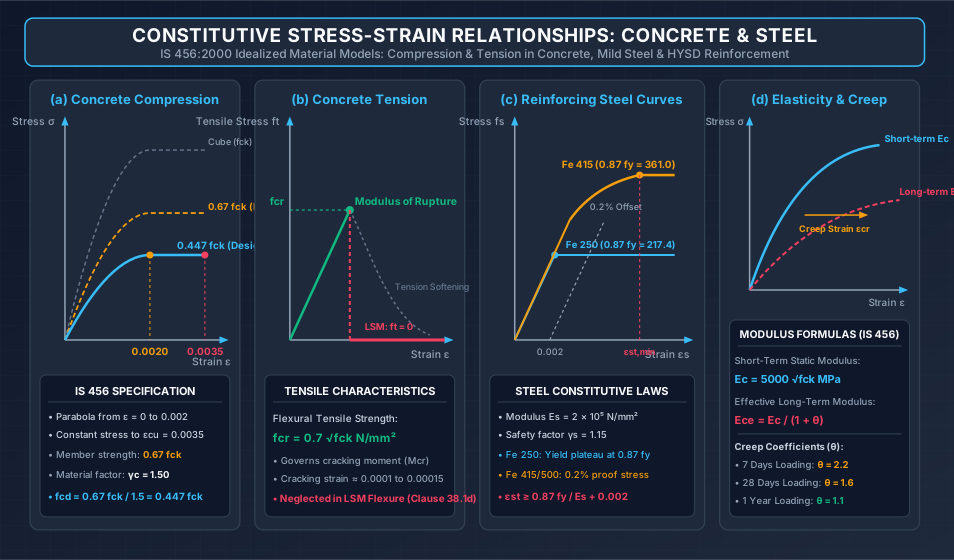
The compressive stress-strain behavior of concrete depends on the specimen boundary conditions, duration of loading, and cross-sectional geometry:
- Standard Cube Curve (): Tested rapidly () in steel platens. Frictional end-restraint generates triaxial compression near the platens, artificially elevating failure strength.
- Structural Member In-Situ Curve (): In an actual full-scale beam or column, platen confinement is absent, member size is larger, and load is sustained over time ( size effect sustained load effect ).
- Design Curve (): Incorporates the material partial safety factor :
The design curve follows the piecewise function:
6.2 Tensile Behavior & Modulus of Rupture
Per IS 456:2000 Clause 6.2.2, the flexural tensile strength (modulus of rupture) is estimated from the standard 28-day cube compressive strength:
- Cracking Moment (): For a gross uncracked section of depth and width :
- Once the outer tensile fiber reaches , tensile micro-cracks form, the concrete relieves tensile stress, and the internal force transfers entirely to the steel reinforcement ().
6.3 Modulus of Elasticity of Concrete
-
Short-Term Static Modulus () (IS 456 Clause 6.2.3.1):
(Note: IS 456:1978 previously specified . This was updated in IS 456:2000 to to reflect modern aggregate and cement formulations).
-
Long-Term Effective Modulus () (IS 456 Clause 6.2.5.1):
Under sustained sustained loading, creep increases concrete strain:where is the Creep Coefficient:
- for loading at 7 days
- for loading at 28 days
- for loading at 1 year
7. Constitutive Stress-Strain Behavior of Reinforcing Steel
7.1 Mild Steel (Fe 250) — Bilinear Model (IS 456 Figure 22)
- Exhibits linear elastic behavior up to yield stress with slope .
- Features a sharp, well-defined yield point at .
- The design curve has yield plateau at:
- Yield strain:
7.2 High-Strength Deformed Bars (Fe 415, Fe 500) — Non-Linear Model (IS 456 Figure 23)
Cold-worked and Thermo-Mechanically Treated (TMT) bars do not exhibit a distinct yield plateau. The curve is idealized into two segments:
- Linear Elastic Range: Strictly linear with slope up to of the design yield strength:
- Non-Linear Transition Range: Beyond , the curve curves monotonically up to the design proof stress , defined by a permanent non-proportional strain offset of ().
Representative Design Stress-Strain Table (SP:16 Table A)
| Steel Stress Level | Total Strain (Fe 415) | Total Strain (Fe 500) |
|---|---|---|
8. Worked Numerical Examples
Problem 1: Integration & Verification of Concrete Stress Block Components
Problem Statement:
A rectangular reinforced concrete beam has width and is cast using M25 grade concrete (). Under ultimate flexure, the depth of the neutral axis is established as .
- Determine the depth of the rectangular and parabolic zones of the compression block.
- Calculate the individual compressive forces developed in the rectangular portion () and parabolic portion ().
- Verify the total compressive force and calculate the precise depth of its line of action () from the extreme top fiber.
Step-by-Step Solution:
Part 1: Depths of Rectangular and Parabolic Zones
- Design compressive stress:
- Depth of rectangular block ():
- Depth of parabolic block ():
Part 2: Compressive Forces and
- Rectangular zone compressive force ():
- Parabolic zone compressive force ():
Part 3: Total Compressive Force and Resultant Centroid
-
Total Compressive Force ():
Comparison with IS 456 codified formula:
(The difference arises from rounding to ).
-
Line of action centroids:
-
Combined centroid ():
Comparison with IS 456 codified formula:
(Matches the exact analytical value ).
Problem 2: Limiting Design Parameters Across Steel Grades
Problem Statement:
A reinforced concrete beam section has width and effective depth . Concrete grade is M25 (). Evaluate and compare the limiting depth of neutral axis (), limiting moment of resistance (), and limiting area of tension reinforcement () for:
- Mild Steel Fe 250
- HYSD Steel Fe 415
- TMT Steel Fe 500
Step-by-Step Solution:
1. Mild Steel Fe 250 ():
- Limiting depth of neutral axis:
- Limiting moment of resistance:
- Limiting area of tension steel:
2. HYSD Steel Fe 415 ():
- Limiting depth of neutral axis:
- Limiting moment of resistance:
- Limiting area of tension steel:
3. TMT Steel Fe 500 ():
- Limiting depth of neutral axis:
- Limiting moment of resistance:
- Limiting area of tension steel:
Comparative Insight:
Transitioning from Fe 250 to Fe 500 decreases the required balanced steel area by (), significantly alleviating reinforcement congestion, with only a nominal drop in the singly reinforced flexural capacity envelope.
Problem 3: Modulus of Rupture & Long-Term Creep Elasticity
Problem Statement:
An RC bridge girder is cast using M30 grade concrete ().
- Calculate the flexural tensile strength (modulus of rupture ).
- Determine the short-term static modulus of elasticity ().
- Evaluate the effective long-term modulus of elasticity () for sustained loading initiated at:
- 7 days of age ()
- 28 days of age ()
- 1 year of age ()
Step-by-Step Solution:
Part 1: Modulus of Rupture ()
Per IS 456:2000 Clause 6.2.2:
Part 2: Short-Term Static Modulus of Elasticity ()
Per IS 456:2000 Clause 6.2.3.1:
Part 3: Long-Term Effective Modulus of Elasticity ()
Per IS 456 Clause 6.2.5.1:
- Loading at 7 Days ():
- Loading at 28 Days ():
- Loading at 1 Year ():
9. Common Misconceptions & Exam Pitfalls
[!WARNING] Pitfall 1: Assuming Depends on Concrete Grade
A widespread error in competitive exams is attempting to calculate using . The limiting depth of neutral axis is derived strictly from strain compatibility ( and ) and depends only on the steel grade .
[!WARNING] Pitfall 2: Confusing with Centroid Measured from Neutral Axis
The factor is measured downwards from the extreme top compression fiber, NOT from the neutral axis. The centroid distance measured up from the neutral axis is .
[!CAUTION] Pitfall 3: Using the Old Modulus Formula ()
In IS 456:1978, the modulus of elasticity of concrete was given as . In IS 456:2000, this was changed to . Using is penalized in all current competitive examinations.
[!IMPORTANT] Pitfall 4: Misapplying the Minimum Steel Strain Formula
Students often forget the offset in the steel yield strain criterion:Omitting produces an erroneous value for .
10. Comparative Summary & Master Formula Sheet
Master Stress Block Parameters (IS 456:2000 Clause 38.1)
| Parameter | Mathematical Expression | Numerical Codified Value |
|---|---|---|
| Peak Concrete Design Stress | ||
| Depth of Rectangular Portion | ||
| Depth of Parabolic Portion | ||
| Total Compressive Force () | ||
| Centroid Depth ( from top) | ||
| Lever Arm () | ||
| Limiting NA Depth Ratio | (Fe 250), (Fe 415), (Fe 500) | |
| Modulus of Rupture | Clause 6.2.2 | |
| Static Modulus of Elasticity | Clause 6.2.3.1 | |
| Effective Long-Term Modulus | Clause 6.2.5.1 |
11. Practice Questions & Competitive Examination Problems
Question 1 (GATE CE — 1 Mark)
In the limit state design of a reinforced concrete beam as per IS 456:2000, the depth of the rectangular portion of the stress block is:
- (A)
- (B)
- (C)
- (D)
Answer: (C)
Explanation: The rectangular portion extends from to the strain level , which occurs at .
Question 2 (UPSC ESE — Objective)
The maximum strain in the tension reinforcement in a balanced reinforced concrete section at collapse should NOT be less than:
- (A)
- (B)
- (C)
- (D)
Answer: (B)
Explanation: IS 456 Clause 38.1(f) mandates .
Question 3 (SSC JE — Technical)
As per IS 456:2000, the limiting value of the depth of neutral axis () for Fe 415 grade steel is:
- (A)
- (B)
- (C)
- (D)
Answer: (B)
Explanation: For Fe 415, .
Question 4 (State AE — Analytical)
If the 28-day characteristic compressive strength of concrete is , the flexural tensile strength and short-term modulus of elasticity as per IS 456:2000 are respectively:
- (A) and
- (B) and
- (C) and
- (D) and
Answer: (A)
Explanation: . .
Question 5 (GATE CE — 2 Marks)
A singly reinforced beam of cross-section (effective depth) is cast with M20 concrete and Fe 415 steel. The limiting moment of resistance () of the section in is:
- (A)
- (B)
- (C)
- (D)
Answer: (B)
Explanation: For Fe 415, .
Question 6 (UPSC ESE — Conventional)
Derive from first principles the expression for the total compressive force and the depth of its line of action for the IS 456:2000 parabolic-rectangular stress block.
Answer Summary: Integrate the rectangular area ( to ) and parabolic area ( to ) to obtain and . Take first moments of area about top fiber to obtain .
12. References & Code Standards
- IS 456:2000 (Reaffirmed 2021): Plain and Reinforced Concrete — Code of Practice, Section 5 (Clause 6: Concrete Properties, Clause 38: Limit State of Collapse — Flexure, Figures 21–24).
- SP:16 (1980): Design Aids for Reinforced Concrete to IS: 456-1978, Bureau of Indian Standards, New Delhi.
- IS 1786:2008: High Strength Deformed Steel Bars and Wires for Concrete Reinforcement — Specification.
- Pillai, S. U., & Menon, D. (2021): Reinforced Concrete Design, 4th Edition, McGraw-Hill Education, India.
- Varghese, P. C. (2009): Limit State Design of Reinforced Concrete, 2nd Edition, PHI Learning Pvt. Ltd., New Delhi.
- Park, R., & Paulay, T. (1975): Reinforced Concrete Structures, John Wiley & Sons.