Tacheometric Surveying, Triangulation Networks & Baseline Extension
In this chapter (1 topics)
On this page
- 1. Module Overview & Pedagogical Scope
- 2. Learning Objectives & Exam Weightage Analysis
- Learning Objectives
- Exam Weightage Analysis
- 3. Tacheometric Optics, Diaphragm Design & Stadia Constants
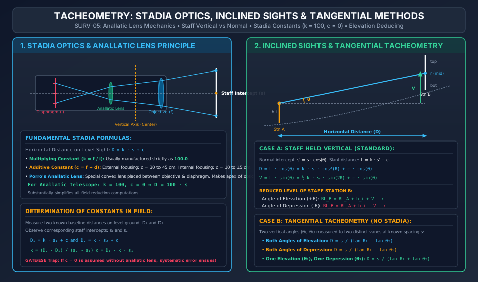
- 3.1 Fundamental Geometry of Stadia Rays
- 3.2 Field Determination of Stadia Constants
- 4. Porro's Anallatic Lens: Optical Geometry & Zero Additive Constant Proof
- 4.1 Optical Architecture
- 4.2 Mathematical Mechanism of c = 0
- 5. Inclined Sights Tacheometry
- 5.1 Case A: Staff Held Vertically (Standard Field Practice)
- 5.2 Case B: Staff Held Normal to the Line of Sight
- 6. Tangential Tacheometry & Subtense Bar Systems
- 6.1 Tangential Tacheometry
- 6.2 Subtense Bar Method (Movable Hair System)
- 7. Triangulation Surveying: Orders & Specifications
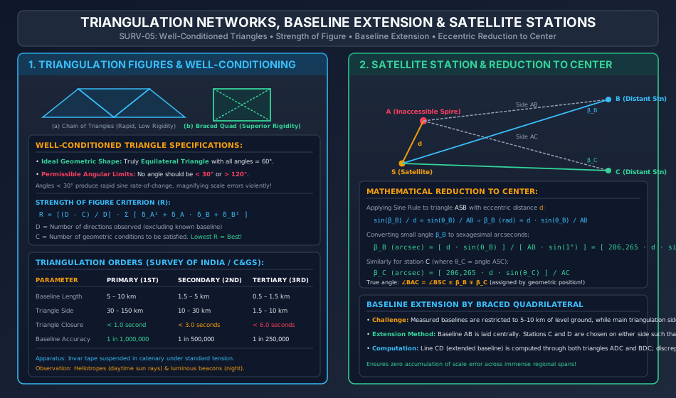
- 7.1 Orders of Triangulation (Survey of India / International Standards)
- 8. Well-Conditioned Triangles & Strength of Figure
- 8.1 Well-Conditioned Triangle Criteria
- 8.2 USC&GS Strength of Figure Criterion (R)
- 9. Baseline Measurement & Extension Schemes
- 9.1 Baseline Measurement
- 9.2 Baseline Extension by Braced Quadrilateral
- 10. Satellite Stations (Eccentric Reduction to Center)
- 10.1 Analytical Derivation
- 10.2 Deduction of True Angle angle BAC
- 11. Step-by-Step Rigorous Worked Numerical Examples
- Problem 1: Stadia Tacheometry with Inclined Sights (Staff Vertical)
- Problem 2: Tangential Tacheometry Across Ravine
- Problem 3: Satellite Station Reduction to Center
- 12. Comprehensive Exam Question Bank
- Section A: GATE CE Previous Years & Anticipated Styles
- Section B: UPSC ESE Conventional Practice
- Section C: SSC JE & State AE/JE Quick Fire
- 13. Common Conceptual Pitfalls & Field Traps
- 14. Quick Reference Formulas & Multi-Code Summary Table
1. Module Overview & Pedagogical Scope
When topographic surveying spans rugged terrains, river canyons, precipitous ravines, or marshlands where direct linear chaining and taping become physically impracticable or prohibitively slow, Tacheometry (tachymetry) and Triangulation serve as the foundational geodetic methodologies.
Tacheometry replaces physical taping with optical distance measurement through an engineered optical telescope fitted with horizontal stadia wires. By reading the intercepted length on a graduated staff and observing the vertical inclination angle, both horizontal distances and vertical elevation differences are resolved simultaneously from a single instrument setup.
Triangulation establishes high-precision national and regional geodetic control frameworks by measuring an initial baseline with extreme precision (historically with invar wires in catenary, now augmented by EDM) and propagating coordinate control across hundreds of kilometers via a rigid network of interconnected triangles whose angles are observed with precision theodolites.
This comprehensive master module synthesizes:
- Optical Mechanics of Stadia Tacheometers: Focal length geometry, stadia interval factor / multiplying constant (), additive constant (), and field determination of constants from baseline calibration.
- Porro's Anallatic Lens: Optical proof of how an internal convex lens eliminates the additive constant (), causing the apex of the measuring angle to coincide identically with the vertical axis of the instrument.
- Inclined Sights Formulations: Mathematical derivations for staff held vertically () versus staff held normal to the line of sight.
- Tangential Tacheometry & Subtense Bar Systems: Distance determination without stadia wires using two vertical angles, and horizontal invar subtense bar principles ().
- Triangulation Figures & Well-Conditioning: Orders of triangulation (Primary, Secondary, Tertiary), angular closures, well-conditioned triangle criteria (, ideal ), and the US Coast and Geodetic Survey (USC&GS) Strength of Figure criterion ().
- Baseline Extension & Satellite Stations (Reduction to Center): Geometric magnification of short baselines via braced quadrilaterals, and analytical reduction of eccentric observations when primary triangulation towers/spires cannot be physically occupied.
2. Learning Objectives & Exam Weightage Analysis
Learning Objectives
- State and derive the fundamental stadia distance formula and prove why an anallatic lens ensures .
- Formulate the exact expressions for horizontal distance () and vertical height () for inclined sights with staff held vertically and deduce reduced levels of staff stations under elevation and depression sights.
- Differentiate between stadia tacheometry, tangential tacheometry, and the subtense bar method in terms of instrument requirements, field procedure, and accuracy.
- Classify triangulation networks into primary, secondary, and tertiary orders according to baseline lengths, triangle side lengths, and permissible triangle closures.
- Apply the Strength of Figure formula () to rank alternative triangulation networks.
- Calculate angular corrections for eccentric satellite stations using the reduction-to-center formula () and resolve true station angles.
Exam Weightage Analysis
| Exam Stream | Typical Question Type | Average Weightage | Recurring Focus Concepts |
|---|---|---|---|
| GATE CE | Numerical Answer Type (NAT) | 1 – 2 Marks | Stadia inclined sight calculations ( and ), anallatic lens properties (), tangential distance formula. |
| UPSC ESE (Prelims & Mains) | Objective + Multi-step Conventional | 10 – 20 Marks | Anallatic lens proof, reduction to center derivation, strength of figure computation, baseline extension schemes. |
| SSC JE / RRB JE | Objective (Conceptual & Formula) | 2 – 4 Questions | Values of and , purpose of anallatic lens, well-conditioned triangle angles ( to ). |
| State PSC AE/JE | Mixed Objective & Short Numerical | 3 – 6 Marks | Formulas for , reduction to center angle signs, primary triangulation closure limits (). |
3. Tacheometric Optics, Diaphragm Design & Stadia Constants
A tacheometer is a transit theodolite fitted with a special diaphragm (reticle) that incorporates two additional horizontal hairs placed symmetrically above and below the central cross-hair, known as stadia hairs.
3.1 Fundamental Geometry of Stadia Rays
Let an external focusing telescope sight a vertical graduated staff held at distance on level ground.
- = Focal length of the objective lens.
- = Distance between the upper and lower stadia hairs (stadia interval on the diaphragm).
- = Intercept on the staff between the upper and lower stadia hair sightlines ().
- = Distance from the optical center of the objective lens to the staff.
- = Distance from the optical center of the objective lens to the diaphragm image.
- = Distance from the optical center of the objective lens to the vertical axis (center) of the instrument.
- = Horizontal distance from the vertical axis of the instrument to the staff ().
From the conjugate focal relationship of a thin lens:
From similar triangles formed by the rays through the optical center:
Substituting into the lens equation:
Adding the mechanical distance from the objective lens to the vertical trunnion axis:
Where:
- = Stadia Interval Factor / Multiplying Constant. In all standard surveying instruments, is manufactured to be exactly .
- = Additive Constant. Represents the distance between the exterior focal point and the instrument center. For ordinary external focusing telescopes, ranges between and ; for internal focusing telescopes, to .
3.2 Field Determination of Stadia Constants
To evaluate and experimentally:
- Lay out a straight baseline on level ground and mark two points at precisely taped distances and from the instrument (e.g., and ).
- Read the corresponding staff intercepts and .
- Set up the two simultaneous linear equations:
- Subtracting gives:
4. Porro's Anallatic Lens: Optical Geometry & Zero Additive Constant Proof
To eliminate the cumbersome additive constant and allow direct calculation of distances via mental arithmetic (), the Italian engineer Ignazio Porro (1823) introduced the Anallatic Lens.
4.1 Optical Architecture
An anallatic lens is an internal convex lens placed between the objective lens and the diaphragm at a precise fixed distance behind the objective.
4.2 Mathematical Mechanism of
When light rays from the staff pass through the objective lens, they converge towards its principal focus. The anallatic convex lens intercepts these converging rays and bends them further so that:
- The virtual vertex (apex) of the measuring optical cone is drawn back to coincide identically with the vertical axis of the instrument.
- The distance between the virtual vertex and the vertical axis becomes zero:
- Therefore:
[!NOTE] An anallatic lens can be fitted only to internal focusing telescopes. While it eliminates the additive constant, it absorbs roughly to of incident light, slightly reducing brightness. Modern Total Stations and electronic digital levels bypass this through coaxial infrared lasers and optoelectronic detectors.
5. Inclined Sights Tacheometry
In rugged terrain, the line of sight must be tilted at an angle of elevation () or depression ().
5.1 Case A: Staff Held Vertically (Standard Field Practice)
Holding the staff vertical with the aid of a plumbing level (circular bubble) attached to the staff is standard practice because keeping a staff truly perpendicular to an inclined line of sight requires a cumbersome mechanical sighting device.
Let the line of sight be inclined at angle to the horizontal.
- The staff is vertical, intercepting length .
- The line normal to the central sightline intercepts length .
- Since is small, the triangle formed by and at the central reading is approximately a right triangle:
The distance along the inclined line of sight () is:
1. Horizontal Distance ():
Projecting the inclined distance onto the horizontal plane:
For an anallatic telescope ():
2. Vertical Component ():
Projecting onto the vertical plane:
For an anallatic telescope ():
3. Reduced Level of Staff Station:
Let:
- = Reduced Level of instrument ground station .
- = Height of the instrument axis above ground peg .
- = Central cross-hair reading on the vertical staff.
- For an Angle of Elevation ():
- For an Angle of Depression ():
5.2 Case B: Staff Held Normal to the Line of Sight
When a special sighting vane is fitted to the staff so the staffman angles it normal to the theodolite sightline:
- Horizontal Distance ():
- For an angle of elevation ():
- For an angle of depression ():
- Vertical Component ():
- For elevation:
- For depression:
6. Tangential Tacheometry & Subtense Bar Systems
6.1 Tangential Tacheometry
Used when an ordinary theodolite without stadia hairs is available, or when distance exceeds the range of readable stadia graduations. Two horizontal targets (vanes) are fixed on the staff at a known vertical separation (e.g., or ). Vertical angles and are measured to the upper and lower targets respectively.
Case 1: Both Angles of Elevation (θ1 > θ2)
        D = s / (tan θ1 - tan θ2)
        V_lower = D * tan θ2

Case 2: Both Angles of Depression (θ2 > θ1)
        D = s / (tan θ2 - tan θ1)
        V_upper = D * tan θ1

Case 3: One Angle of Elevation (θ1) and One Angle of Depression (θ2)
        D = s / (tan θ1 + tan θ2)
        V_upper = D * tan θ1,   V_lower = D * tan θ2
6.2 Subtense Bar Method (Movable Hair System)
A horizontal bar of fixed length (usually of invar steel) is mounted horizontally on a tripod at the target station, perpendicular to the line of sight.
- The theodolite measures the horizontal angle subtended by the ends of the bar.
- Distance is computed directly from right-triangle trigonometry:
- Crucial Advantage: Because is measured strictly in the horizontal circle, the computed distance is automatically the true horizontal distance, completely independent of the vertical inclination of the terrain!
7. Triangulation Surveying: Orders & Specifications
Triangulation consists of measuring the length of one baseline and computing all other side lengths throughout the network by measuring the interior angles of interconnected triangles using the Sine Rule:
7.1 Orders of Triangulation (Survey of India / International Standards)
| Order / Class | Typical Baseline Length | Triangle Side Length | Average Triangle Angular Closure | Max Permissible Angular Closure | Baseline Precision |
|---|---|---|---|---|---|
| Primary (1st Order) | |||||
| Secondary (2nd Order) | |||||
| Tertiary (3rd Order) |
8. Well-Conditioned Triangles & Strength of Figure
8.1 Well-Conditioned Triangle Criteria
Errors in measured angles propagate into calculated side lengths through their sines. Differentiating :
- When an angle approaches or , , causing explosive magnification of errors!
- Ideal Geometric Form: The Equilateral Triangle (), where error propagation is at an absolute minimum.
- Permissible Field Limits: No triangle angle should ever be or .
8.2 USC&GS Strength of Figure Criterion ()
To quantitatively select the strongest chain among competing route alignments:
Where:
- = Number of direction observations made in the figure (excluding the known baseline).
- = Number of geometric conditions that must be satisfied in the figure:
- = Total number of lines.
- = Number of lines observed in both directions.
- = Total number of stations.
- = Number of stations occupied.
- = Tabular difference for in the log sine of distance angles and (angles opposite the unknown and known sides in each triangle).
- Selection Rule: The layout yielding the lowest value of possesses the greatest mathematical rigidity and accumulates the minimum error.
9. Baseline Measurement & Extension Schemes
9.1 Baseline Measurement
Baselines are measured along smooth, flat terrain using invar tapes () suspended in catenary (air) under standardized tension applied via frictionless pulleys or weights. All 6 fundamental corrections (standard length, temperature, pull, sag, slope, and reduction to mean sea level) are applied.
9.2 Baseline Extension by Braced Quadrilateral
Because terrain rarely allows a directly taped baseline longer than , while primary triangle sides span , the baseline must be magnified optically:
- Short baseline is measured accurately in a flat valley.
- Stations and are established on high ridges on either side, forming braced quadrilateral .
- All internal angles and diagonals and are observed.
- The extended baseline length is computed independently through and . The agreement confirms magnification without loss of precision.
10. Satellite Stations (Eccentric Reduction to Center)
In triangulation, primary stations are frequently selected on prominent summits, church spires, lighthouse beacons, or high water towers to provide line of sight over curvature and obstructions. However, a theodolite cannot be centered over an inaccessible spire or atop a narrow pinnacle.
In such cases, an eccentric station / satellite station () is established at a short distance from the true center station (). Angles observed at must be corrected mathematically to obtain the angles that would have been measured at true center —a process termed Reduction to Center.
10.1 Analytical Derivation
Let:
- = True inaccessible triangulation station (center).
- = Eccentric satellite station occupied by the instrument.
- = Measured eccentric distance between and (usually measured to the millimeter with a steel tape).
- = Distant triangulation targets.
- = Distances to targets (approximated from preliminary triangulation computations or map data; extreme precision in is not required because ).
- = Observed angle from baseline to distant station .
- = Small angular correction at distant station .
Applying the Sine Rule to :
Because is extremely small (a few arcseconds), :
Converting radians to sexagesimal arcseconds by dividing by :
Similarly, for distant station (where ):
10.2 Deduction of True Angle
By resolving the geometry of the four-point figure :
(The algebraic signs or are governed strictly by whether lies to the left or right of the lines of sight).
11. Step-by-Step Rigorous Worked Numerical Examples
Problem 1: Stadia Tacheometry with Inclined Sights (Staff Vertical)
Problem Statement:
A tacheometer fitted with an anallatic lens () is set up at station having a Reduced Level . The height of the instrument axis above the station peg is .
A sight is taken to a staff held vertically at station . The vertical angle is (angle of elevation).
The staff readings intercepted by the stadia hairs are:
- Top hair
- Middle (axial) hair
- Bottom hair
Calculate:
- Staff intercept and confirm middle hair symmetry.
- The horizontal distance between station and station .
- The vertical elevation difference between the trunnion axis and the central hair.
- The Reduced Level of station .
Step 1: Staff Intercept and Check
Symmetry check:
Axial reading .
Step 2: Compute Horizontal Distance ()
Given: .
Using the inclined sight formula for vertical staff:
Since anallatic lens is fitted, :
Step 3: Compute Vertical Component ()
Step 4: Compute Reduced Level of Station
Because the sight is an angle of elevation ():
Problem 2: Tangential Tacheometry Across Ravine
Problem Statement:
To determine the distance to an inaccessible bench mark across a deep mountain ravine, a theodolite is set up at station (, instrument height ). An ordinary metric staff is held vertically at .
Two targets fixed on the staff at and above the ground are sighted:
- Angle of elevation to upper target ():
- Angle of elevation to lower target ():
Compute:
- The horizontal distance from to .
- The Reduced Level of station .
Step 1: Geometry and Intercept
- Distance between vanes on staff:
- Tangents of vertical angles:
Step 2: Calculate Horizontal Distance ()
Step 3: Calculate Vertical Height and RL of Station
The height of the lower target above the instrument axis is:
Check using upper target:
Note: [Check verified!].
The lower vane is above ground level at :
Problem 3: Satellite Station Reduction to Center
Problem Statement:
In a major geodetic triangulation network, primary station is an inaccessible church spire. A satellite station was set up at an eccentric distance from .
From station , sighting back to and to two distant triangulation targets and yielded the following observed horizontal angles:
(Station lies to the left of both lines of sight and ).
The approximate distances to the distant stations are:
Calculate the corrected true horizontal angle at the primary triangulation station .
Step 1: Determine Observed Angles from Baseline
- Angle to target :
- Angle to target :
Step 2: Compute Small Angle Corrections and
Formula: where :
-
For Station :
Converting to minutes and seconds:
-
For Station :
Converting to minutes and seconds:
Step 3: Determine True Angle
Since satellite station lies to the left of both rays:
- The ray from true station to is rotated clockwise relative to by :
- The ray from true station to is rotated clockwise relative to by :
Therefore:
Substituting the numerical values:
12. Comprehensive Exam Question Bank
Section A: GATE CE Previous Years & Anticipated Styles
-
[GATE CE] The multiplying constant and additive constant of a tacheometer are and respectively. An inclined sight was taken to a vertically held staff at an angle of elevation of . If the staff intercept is , the horizontal distance between the instrument and the staff is:
- (A)
- (B)
- (C)
- (D)
Answer: (B). .
-
[GATE CE] An anallatic lens provided in a tacheometer:
- (A) Increases the magnification of the image
- (B) Makes the additive constant zero
- (C) Makes the multiplying constant zero
- (D) Eliminates the effect of earth curvature
Answer: (B).
Section B: UPSC ESE Conventional Practice
- [ESE Mains] In a triangulation survey, define what is meant by a 'Satellite Station' and deduce the formula for reduction to center when the satellite station is located to the right of the survey line. Discuss the precautions taken during baseline extension by braced quadrilaterals.
Section C: SSC JE & State AE/JE Quick Fire
- In subtense bar tacheometry, the distance determined is:
- (A) Slant distance along the line of sight
- (B) Directly the horizontal distance, irrespective of terrain slope
- (C) Dependent on staff verticality errors
- (D) Affected by refraction curvature corrections
Answer: (B).
- For a well-conditioned triangle in triangulation, no interior angle should be less than:
- (A)
- (B)
- (C)
- (D)
Answer: (B) .
- In a primary triangulation network, the maximum permissible average triangle angular closure is:
- (A)
- (B)
- (C)
- (D)
Answer: (A) .
13. Common Conceptual Pitfalls & Field Traps
- Staff Normal vs Staff Vertical Formula Trap:
Applying when the staff is held normal to the line of sight.
Field Reality: When the staff is held normal, the intercept is already perpendicular to the line of sight, so , and the horizontal distance is (only single power of ). - Satellite Station Sign Misassignment:
Applying a fixed mnemonic for in satellite reduction without sketching the geometry.
Field Reality: Always sketch the eccentric point and true point . If ray is to the left of the target, true azimuth from is larger/smaller based on whether line crosses the line of sight. - Anallatic Lens Additive Constant Trap:
Assuming for all modern theodolites. Unless explicitly specified that an internal focusing telescope has an anallatic lens, is typically . - Middle Hair Symmetry Error:
Failing to check that . If this does not hold within , either the stadia diaphragm has displaced or a staff reading was recorded incorrectly.
14. Quick Reference Formulas & Multi-Code Summary Table
| Category | Parameter | Exact Analytical Formulation |
|---|---|---|
| Stadia Level Sight | Distance () | () |
| Stadia Inclined (Staff Vertical) | Horizontal Distance () | |
| Vertical Height () | ||
| RL (Elevation ) | ||
| RL (Depression ) | ||
| Anallatic Telescope | Distance () | |
| Vertical Height () | ||
| Tangential Tacheometry | Distance () | |
| Distance () | ||
| Subtense Bar | Horizontal Distance () | |
| Triangulation Conditioning | Ideal Triangle | Equilateral () |
| Allowable Angle Limits | ||
| Strength of Figure | Rigidity Index () | |
| Satellite Station | Angular Correction () | |
| True Center Angle |