Fundamental Principles, Precision, Error Theory & Linear Measurements — Chaining, Taping & Precision Baseline Corrections
In this chapter (1 topics)
On this page
- 1. Module Overview & Technical Architecture
- 2. Governing Formulae, Empirical Relations & Code Provisions
- 2.1 Metric Chains & Standardization Standards (IS 1492)
- 2.2 Traditional Non-Metric Chains (Historical & Land Revenue Standards)
- 2.3 The Six Systematic Baseline Tape Corrections
- 2.4 Theory of Errors & Precision Indices (Gaussian Statistics)
- 3. Step-by-Step Analytical Derivations & Mechanisms
- 3.1 Plumb Line Convergence & Spherical Excess Derivation
- 3.2 Analytical Derivation of the Sag Correction (Cs)
- 3.3 Normal Tension (Pn) Formulation
- 3.4 Series Expansion for Slope Correction (Cg)
- 4. Classification of Surveying: Plane vs Geodetic Surveying
- 5. Theory of Errors, Precision, Accuracy & Most Probable Value
- 5.1 Distinction: Precision vs Accuracy vs Discrepancy
- 5.2 Classification of Measurement Errors
- 5.3 Mathematical Laws of Weights
- 6. Linear Measurements: Instruments, Metric Chains & Stepping on Slopes
- 6.1 Tapes: Materials & Metallurgical Precision
- 6.2 Chaining on Sloping Ground
- 7. The Six Standard Tape Corrections & Precision Baselines
- 7.1 Sequence of Physical Reductions
- 8. Field Obstacles in Chaining & Vision
- 9. Embedded Technical Visualizations & Diagrams
- 9.1 Surveying Principles, Plane vs Geodetic & Error Theory
- 9.2 Chaining Mechanics, Stepping Method & The Six Baseline Tape Corrections
- 10. Worked Analytical & Design Numerical Problems
- Problem 1: Precision Geodetic Baseline Tape Corrections
- Problem 2: Theory of Errors, Weights & Most Probable Value
- Problem 3: Chaining on Sloping Ground with an Erroneous Chain
- 11. Cross-Exam Synthesis Matrix
- 12. Common Failure Modes, Systematic Field Biases & Forensic Engineering
- 12.1 Erroneous Tape Standardization & Cumulative Scale Bias
- 12.2 Temperature Gradient Bias & Catenary Wind Flutter
- 13. Practice Problems & Exam Drill Questions
- Question 1 (GATE Style — NAT)
- Question 2 (UPSC ESE Style — Conceptual Multiple Choice)
- Question 3 (SSC JE / RRB JE Style — Quick Recall)
- 14. Comprehensive Technical Reference & Cross-Topic Linkages
- Inter-Topic Knowledge Mapping
- Standard Code References
1. Module Overview & Technical Architecture
Surveying is the foundational science, art, and technology of determining the relative spatial positions of points above, on, or beneath the Earth's surface by means of direct or indirect measurements of distance, direction, and elevation. It forms the indispensable prerequisite for all civil engineering endeavors — from route reconnaissance, corridor alignment, and topographic mapping to structural setting-out, dimensional verification, and crustal deformation monitoring.
The technical architecture of surveying rests on two axiomatic principles:
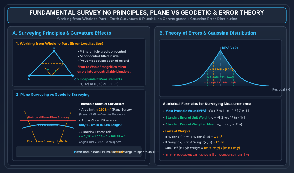
- Working from Whole to Part: Establishing an expansive, high-precision primary control network (triangulation, trilateration, or primary traverse) covering the entire project perimeter, followed by progressive densification into secondary, tertiary, and local minor detail loops. This strategy ensures that local operational errors are rigidly confined within their parent control blocks, preventing runaway accumulation and propagation of measurement errors across the project domain.
- Fixing Positions by at Least Two Independent Reference Measurements: Every new spatial point must be located relative to at least two established, verified reference stations through independent geometric observables (e.g., two linear distances, two horizontal directions, one distance and one bearing, or perpendicular offsets).
                            SURVEYING EXECUTION HIERARCHY
                                          │
                 ┌────────────────────────┴────────────────────────┐
                 ▼                                                 ▼
          PLANE SURVEYING                                  GEODETIC SURVEYING
   • Earth curvature neglected (Flat datum)         • Earth spheroidal curvature included
   • Plumb lines assumed strictly parallel          • Plumb lines converge to Earth's centre
   • Area threshold < 250 km²                       • Area threshold > 250 km²
   • Arc vs Chord error < 1 cm in 18.5 km           • Geodetic baseline & satellite geodesy
   • Spherical excess < 1.0" in 195.5 km²           • True spheroidal triangle computations

                                MEASUREMENT PHYSICS
                                          │
                 ┌────────────────────────┴────────────────────────┐
                 ▼                                                 ▼
         LINEAR MEASUREMENTS                               ANGULAR MEASUREMENTS
   • Direct Chaining & Taping (Metric chains)       • Prismatic & Surveyor's Compasses
   • Electronic Distance Measurement (EDM)          • Optical & Electronic Theodolites
   • Subtense Bar & Stadia Tacheometry              • Total Stations & Robotic EDM
   • 6 Systematic Tape Corrections                  • Astronomical & Gyroscopic Azimuths
2. Governing Formulae, Empirical Relations & Code Provisions
2.1 Metric Chains & Standardization Standards (IS 1492)
Indian Standards (IS 1492) define standard metric chains manufactured from galvanized mild steel wire ( dia) with brass swivel handles at both ends:
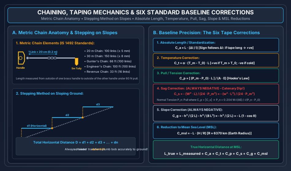
- Metric Chain: Divided into of () each. Equipped with brass tallies at every (1-tooth tally at and , 2-tooth tally at , rounded groove at center ).
- Metric Chain: Divided into of each. Tallies provided at every ().
- Standard Pull & Temperature: Chains are standardized under a pull of () at a standard temperature of .
- Permissible Manufacturing Tolerances (IS 1492):
- chain: Within .
- chain: Within .
- Length of an individual link: Within .
2.2 Traditional Non-Metric Chains (Historical & Land Revenue Standards)
- Gunter's Chain (Surveyor's Chain): Length = , containing (). Convenient for land acreage: (); ().
- Engineer's Chain: Length = , containing ().
- Revenue Chain: Length = , containing (). Used in cadastral surveys.
2.3 The Six Systematic Baseline Tape Corrections
| Correction Type | Governing Equation | Algebraic Sign | Primary Physical Variables |
|---|---|---|---|
| 1. Absolute Length / Standardization () | = actual tape length, = nominal length, . (+ve if tape too long; -ve if too short). | ||
| 2. Temperature () | = thermal expansion coefficient ( for steel, for Invar), = field temp, = standardization temp. | ||
| 3. Pull / Tension () | = applied field pull, = standard pull (), = tape cross-section, = Young's modulus (). | ||
| 4. Sag () | ALWAYS NEGATIVE () | = total weight of tape between supports, = weight per unit length, = field pull. | |
| 5. Slope () | ALWAYS NEGATIVE () | = vertical elevation difference between tape ends, = slope angle to horizontal. | |
| 6. Mean Sea Level Reduction () | ALWAYS NEGATIVE () | = mean elevation of baseline above MSL, = mean radius of Earth. |
2.4 Theory of Errors & Precision Indices (Gaussian Statistics)
- Most Probable Value (MPV) for weighted observations:
- Residual (): .
- Standard Error of Unit Weight ():
- Standard Error of the Weighted Mean ():
- Probable Error of a Single Observation ():
- Probable Error of the Mean ():
3. Step-by-Step Analytical Derivations & Mechanisms
3.1 Plumb Line Convergence & Spherical Excess Derivation
Consider three geodetic stations on the spherical surface of the Earth forming a large spherical triangle of area , with Earth radius .
- Plumb lines at any two surface stations separated by arc distance are oriented along the local normals to the geoid, both pointing directly toward the Earth's geometric center .
- The central angle subtended at the Earth's center is:
- For an arc length and :
- Chord distance between the two points: .
- Arc-to-chord discrepancy:
- Spherical Excess (): The sum of interior angles of a spherical triangle exceeds Euclidean flat-plane geometry () by the spherical excess : By Girard's Theorem on a sphere: Converting to angular seconds (), where :
3.2 Analytical Derivation of the Sag Correction ()
When a surveying tape of length and weight per unit length is suspended horizontally between two supports under tension , it sags into a catenary curve:
Where parameter . For small dips typical in surveying (), the catenary is closely approximated by a second-degree parabola:
 Support A                                              Support B
     ▼                                                      ▼
     ├──────────────────────────────────────────────────────┤  <- Chord L_chord
      \                                                    /
       \                      Dip d                       /
        \                       ▼                        /
         '──────────────────────●───────────────────────'  <- Curved Tape Length L
- The differential arc length along the sagged curve is:
- Using binomial expansion since :
- Differentiating with the origin at the lowest mid-span point (spanning from to ):
- Integrating across the span from to :
- The sag correction is the negative difference between the straight chord distance () and the curved tape length (): (For a tape supported at equal bays of length with bay weight , the total sag correction is: . Thus, supporting a tape at spans reduces sag error by a factor of !).
3.3 Normal Tension () Formulation
Normal tension () is the theoretical pull applied in the field such that the positive elongation caused by tension () exactly balances and nullifies the negative shortening caused by sag ():
Canceling length and rearranging:
Taking the square root on both sides:
(Solved iteratively for in baseline survey design).
3.4 Series Expansion for Slope Correction ()
Consider a tape stretched along a ground slope of angle over inclined length , with vertical height difference between ends:
- True horizontal distance: .
- Expanding binomially:
- The slope correction is : (For slopes where or , the first term provides millimeter precision).
4. Classification of Surveying: Plane vs Geodetic Surveying
The fundamental operational distinction in surveying hinges on whether the curvature of the Earth is treated as negligible (Plane Surveying) or explicitly parameterized as an oblate spheroid (Geodetic Surveying).
| Characteristic Feature | Plane Surveying | Geodetic Surveying |
|---|---|---|
| Datum Geometry | Earth's surface assumed to be a geometric flat plane. | Earth modeled as an ellipsoid of revolution (WGS-84 / GRS-80). |
| Plumb Line Direction | Plumb lines at any two adjacent stations are assumed strictly parallel. | Plumb lines are normal to the geoid and converge to Earth's centre. |
| Area Threshold | Projects with planar area (). | Large geographic surveys spanning . |
| Line Geometry | Triangles formed are Euclidean plane triangles (). | Triangles are spherical triangles (). |
| Surveying Methodology | Direct chaining, compass traversing, ordinary optical levelling. | High-precision baseline Invar taping, GNSS geodesy, precise gravimetry. |
| Agency Responsible | State PWDs, Municipal Corporations, Private Civil Contractors. | Survey of India (SOI), National Geodetic Survey (NGS). |
5. Theory of Errors, Precision, Accuracy & Most Probable Value
5.1 Distinction: Precision vs Accuracy vs Discrepancy
- Precision: Refers to the degree of repeatability, refinement, and mutual closeness among repeated independent observations made under identical operational conditions. It is governed purely by random dispersion and instrument sensitivity.
- Accuracy: Refers to the absolute closeness of an observation (or the mean of observations) to the true value of the measured quantity. High precision does not guarantee accuracy if an uncorrected systematic bias exists.
- Discrepancy: The numerical difference between two independent measurements of the same physical quantity.
5.2 Classification of Measurement Errors
- Gross Errors (Blunders / Mistakes):
- Caused by human carelessness, confusion, or misreading (e.g., recording instead of , transposing digits, reading the wrong tally).
- Treatment: Not subject to statistical analysis; detected and eliminated by independent checks and field repetitions.
- Systematic Errors (Cumulative Errors):
- Constant or mathematically predictable biases following definite physical or deterministic laws (e.g., tape expansion from heat, erroneous chain length, sag, refraction).
- Mathematical Law: Because systematic errors persist with constant sign per unit length, the total error accumulates linearly:
- Treatment: Completely eliminated or minimized by applying analytical physical corrections ().
- Random Errors (Accidental / Compensating Errors):
- Uncontrollable, non-deterministic residual variations arising from human sensory limits, ambient atmospheric turbulence, and microscopic mechanical imperfections.
- Mathematical Law: Governed by Gaussian normal distribution; positive and negative errors occur with equal probability and partially cancel out:
                 TYPES OF SURVEYING ERRORS & PROPAGATION
                                    │
         ┌──────────────────────────┼──────────────────────────┐
         ▼                          ▼                          ▼
    GROSS ERRORS             SYSTEMATIC ERRORS           RANDOM ERRORS
  (Carelessness)               (Physical Bias)       (Gaussian Fluctuations)
  • Eliminated by            • Law: E ∝ L              • Law: E ∝ √L
    checks & repeats         • Corrected by equations  • Treated statistically
5.3 Mathematical Laws of Weights
The weight () of an observation quantifies its relative trustworthiness or precision, inversely proportional to the variance ():
- Weight of a Product: If an observation has weight , then the quantity has weight:
- Weight of a Quotient:
- Weight of Linear Combination: If has weight and has weight :
- Weight of an Observation of Weight Multiplied by a Negative Sign:
6. Linear Measurements: Instruments, Metric Chains & Stepping on Slopes
6.1 Tapes: Materials & Metallurgical Precision
- Cloth / Linen Tape: Woven linen varnished to resist moisture; stretches severely under tension and rots when damp; suitable only for rough architectural offsets.
- Metallic Tape: Linen tape reinforced with interwoven fine brass or copper bronze wires; reduces stretching; suitable for ordinary engineering surveys.
- Steel Tape: Ribbon of cold-rolled high-carbon tempered spring steel ( width); highly accurate, but prone to rust and brittle snapping if kinked.
- Invar Tape: Alloy composed of Nickel and Steel; exhibits an exceptionally low coefficient of thermal expansion (, less than one-tenth of steel); used universally for national geodetic triangulation baselines; highly soft, expensive, and fragile.
6.2 Chaining on Sloping Ground
When measuring linear distances across undulating or sloping topography, the true horizontal projection must be recorded:
- Direct Method (Stepping Method / Drop Chaining):
- The tape is stretched horizontally in convenient, short step increments (, typically ) depending on the steepness of the terrain.
- The downhill end is transferred vertically to the ground surface using a plumb bob.
- Chaining is executed strictly downhill because the rear surveyor anchors the tape at ground level while the forward surveyor holds the tape elevated horizontally, sighting the plumb line accurately.
- Total horizontal distance: .
- Indirect Method (Angle of Slope / Elevation Difference):
- The sloping distance () along the ground surface is measured with chain/tape, and the slope angle () is measured with an Abney level, clinometer, or theodolite.
- Horizontal distance: .
7. The Six Standard Tape Corrections & Precision Baselines
In geodetic surveys, city control surveys, and precision structural grids, linear base measurements must be corrected sequentially for all physical and environmental variations:
7.1 Sequence of Physical Reductions
- Absolute Length Correction (): Accounts for the manufactured deviation of the tape from its nominal reference length:
- Temperature Correction (): Accounts for thermal expansion or contraction relative to the calibration datum:
- Pull Correction (): Accounts for elastic Hookean elongation when applied field tension differs from calibration pull:
- Sag Correction (): Compensates for the shortened chord distance when the tape hangs in an unsupported catenary:
- Slope Correction (): Projects inclined surface measurements onto a true horizontal plane:
- Mean Sea Level (MSL) Reduction (): Reduces the horizontal measurement at elevation to the spherical reference geoid:
8. Field Obstacles in Chaining & Vision
Obstacles encountered during linear chain surveys are classified into three distinct physical categories:
                          CLASSIFICATION OF OBSTACLES
                                       │
         ┌─────────────────────────────┼─────────────────────────────┐
         ▼                             ▼                             ▼
   OBSTACLES TO CHAINING        OBSTACLES TO VISION        OBSTACLES TO BOTH
    (Vision Free, Chaining      (Chaining Free, Vision     (Neither Vision nor
          Obstructed)                Obstructed)          Chaining Possible)
  • Rivers, ponds, deep       • High sand dunes, hills,   • Tall multi-storey
    chasms, dense marshes       dense tree groves           buildings, warehouses
- Obstacles to Chaining Only (Rivers, Ponds):
- The line of sight across the river or pond is unobstructed, but chaining directly across water is impossible.
- Geometric Solutions:
- Right-Angle Offset Method: Construct perpendicular line along the river bank; set out an equilateral or right-angled triangle using a cross-staff or optical square ().
- Congruent Triangle Method: Prolong tie lines to create congruent geometric triangles on firm ground.
- Obstacles to Vision Only (Hills, Elevated Mounds):
- The ends of the survey line are not mutually intervisible, but chaining can be performed along the intervening ground.
- Solution: Reciprocal Ranging (Random Line Method) using two surveyors equipped with ranging rods alternately aligning each other on the hillcrest until both lie exactly on the true line .
- Obstacles to Both Vision and Chaining (Buildings):
- Neither line of sight nor linear chaining can penetrate the obstacle.
- Solutions:
- Construct a parallel auxiliary line clear of the building by erecting equal perpendicular offsets ().
- Construct an equilateral triangle or rectangular detour around the structure.
9. Embedded Technical Visualizations & Diagrams
9.1 Surveying Principles, Plane vs Geodetic & Error Theory
The fundamental principle of working from whole to part, the geometry of Earth curvature with converging plumb lines, and the Gaussian normal error distribution are illustrated below.
9.2 Chaining Mechanics, Stepping Method & The Six Baseline Tape Corrections
The detailed mechanical anatomy of metric chains, the stepping method on slopes, and the complete physics governing the six standard tape corrections are presented below.
10. Worked Analytical & Design Numerical Problems
Problem 1: Precision Geodetic Baseline Tape Corrections
Statement: A precision geodetic baseline is measured using a standardized steel tape. The total measured baseline distance is recorded as ( full tape lengths). The tape calibration certificate specifies:
- Nominal length .
- True length under standard pull and temperature on flat support is ().
- Cross-sectional area .
- Modulus of elasticity .
- Coefficient of thermal expansion .
- Total weight of the tape in air .
During field baseline measurement:
- Mean field temperature .
- Applied field tension .
- The tape was suspended in equal spans of each per tape length ( equal bays across the baseline).
- The average ground elevation of the baseline above Mean Sea Level (MSL) is .
- Earth radius .
Compute:
- Absolute length correction ().
- Temperature correction ().
- Pull / tension correction ().
- Total sag correction ().
- Reduction to Mean Sea Level ().
- Total net correction and the true horizontal geodetic baseline length at MSL ().
Analytical Solution:
Step 1: Absolute Length / Standardization Correction ()
Step 2: Temperature Correction ()
Step 3: Pull / Tension Correction ()
Step 4: Total Sag Correction () The baseline contains tape lengths, each suspended in equal bays (). Total number of bays across the baseline . Weight of each bay:
Sag correction for one bay:
Total sag correction for all 36 bays:
Step 5: Reduction to Mean Sea Level ()
Step 6: Net Correction and True Baseline Length ()
Problem 2: Theory of Errors, Weights & Most Probable Value
Statement: An angle was measured independently by four different surveying parties with varying field equipment and repetitions, yielding the following results:
- Observation 1: (Weight )
- Observation 2: (Weight )
- Observation 3: (Weight )
- Observation 4: (Weight )
Determine:
- The Most Probable Value (MPV) of the angle.
- The residuals () for each observation.
- The standard error of unit weight ().
- The standard error of the weighted mean ().
- The probable error of the weighted mean ().
Analytical Solution:
Step 1: Most Probable Value (MPV) Let the base angle be . The observed seconds values are: , , , . Weights: , , , .
Step 2: Residuals () & Weighted Squared Residuals
Step 3: Standard Error of Unit Weight () Number of observations :
Step 4: Standard Error of the Weighted Mean ()
Step 5: Probable Error of the Weighted Mean ()
Problem 3: Chaining on Sloping Ground with an Erroneous Chain
Statement: A distance measured along sloping ground with a nominal metric chain is recorded as . Upon testing the chain against a standardized test bench, it was discovered that the chain was too long (). The field slope profile comprised:
- First of measured length had a uniform slope of ().
- Remaining of measured length had a measured slope angle of ().
Determine the true horizontal ground distance between the survey stations.
Analytical Solution:
Step 1: Correction for Chain Length Error Because the chain is too long ( instead of ), each nominal chain length actually covered .
- True slope distance for Stretch 1:
- True slope distance for Stretch 2:
Step 2: Horizontal Projection for Stretch 1 ()
Step 3: Horizontal Projection for Stretch 2 ()
Step 4: Total True Horizontal Ground Distance ()
11. Cross-Exam Synthesis Matrix
| Exam | High-Frequency Conceptual Focus | Typical Calculation Types | Priority Traps & Critical Nuances |
|---|---|---|---|
| GATE CE | • Sag catenary derivation () • Normal tension iterative equation () • Most probable value with weights • Laws of weights (, weight of ) |
• Multi-span baseline sag calculation • True horizontal distance across multiple slopes • Standard error of unit weight vs mean |
• Sag correction is ALWAYS NEGATIVE; pull correction can be positive or negative! • In sag formula, distinguish between total weight and weight per unit length () • When a tape is supported in equal bays, sag correction is reduced by ! |
| UPSC ESE | • Full analytical derivation of slope series () • Derivation of spherical excess () • Normal tension derivation () • Obstacles in chaining (geometry of congruent triangles) |
• Conventional 15-mark geodetic baseline reductions • Weighted least-squares angle adjustments • Invar baseline precision calculations |
• Remember to apply MSL reduction (); often forgotten in baseline problems • For Invar tape, thermal coefficient is lower than steel • Plumb lines are NOT parallel in geodetic surveying. |
| SSC JE / RRB JE | • Permissible chain tolerances ( for , for ) • Number of links in metric chains ( and ) • Gunter's chain () • Stepping method (downhill chaining with plumb bob) |
• True distance with erroneous chain () • Slope correction first term () • Temperature correction sign check |
• If chain is "too long", measured distance is "too short", so correction is POSITIVE! • in metric chains; in Gunter's chain • Revenue chain has 16 links for . |
| State AE / PSU | • Principles of surveying (Whole to part, 2 independent measurements) • Plane vs Geodetic threshold () • Arc vs chord discrepancy ( in ) • Systematic () vs Random () |
• Quick calculation of true area () • True volume () • Weight of linear equation () |
• True Area is proportional to , NOT ! • True Volume is proportional to ! • Working from part to whole is a FATAL surveying error. |
12. Common Failure Modes, Systematic Field Biases & Forensic Engineering
12.1 Erroneous Tape Standardization & Cumulative Scale Bias
- Failure Phenomenon: A major linear highway or railway baseline survey executed with an uncalibrated field steel tape results in systematic boundary encroachment and structural misfits at bridge abutments and tunnel portals.
- Root Cause & Forensic Diagnosis:
- Steel tapes worn down at the brass hook or stretched past elastic yield during rough field clearing exhibit a persistent elongation error.
- Across a alignment, an uncorrected error per tape accumulates systematically to:
- Forensic Countermeasures:
- Daily calibration against a certified permanent quartz/Invar field comparator base.
- Laser interferometer or electronic total station frequency verification.
12.2 Temperature Gradient Bias & Catenary Wind Flutter
- Failure Phenomenon: High-tension geodetic baseline taping across sunlit asphalt roads exhibits unexplainable closing errors.
- Micro-climate Dynamics: Ground asphalt radiates thermal heat, creating a localized vertical temperature gradient of within of the surface. A handheld thermometer reading ambient air at eye level underestimates true tape temperature by , inducing large systematic negative baseline scale errors.
- Field Protocol: Use embedded digital contact thermocouples affixed directly to the tape ribbon.
13. Practice Problems & Exam Drill Questions
Question 1 (GATE Style — NAT)
A steel tape weighing has a cross-sectional area of . The tape was standardized on the flat under a pull of . If the tape is used in the field suspended in a single catenary span between supports under a pull of , determine the normal tension (in ) required to completely eliminate sag correction if . (Take ).
- Answer:
- Explanation:
- Total tape weight .
- Area .
- .
- Normal tension relation: .
- .
- Solving :
- For : (too high).
- Let's check : .
- For : .
- For : .
Question 2 (UPSC ESE Style — Conceptual Multiple Choice)
Consider the following statements regarding Linear Measurements and Surveying Principles:
- Working from whole to part ensures that errors are localized and prevented from accumulating.
- In plane surveying, plumb lines at different points are assumed to be parallel.
- The sag correction for a tape suspended in catenary is always negative.
- If an observation has weight , then the weight of the quantity is .
Which of the above statements are CORRECT?
- Options: (a) 1, 2, and 3 only (b) 1, 3, and 4 only (c) 2 and 4 only (d) 1, 2, 3, and 4
- Correct Answer: (a) 1, 2, and 3 only
- Explanation: Statement 4 is incorrect because by the mathematical laws of weights, . Thus, the weight of is (not ). Statements 1, 2, and 3 are entirely correct.
Question 3 (SSC JE / RRB JE Style — Quick Recall)
A line was measured with a chain and found to be . If the chain was actually too long, the true length of the line is:
- Options: (a) (b) (c) (d)
- Correct Answer: (b) 502.5 m
- Explanation: .
14. Comprehensive Technical Reference & Cross-Topic Linkages
Inter-Topic Knowledge Mapping
- Upstream Linkages:
SOM-01: Hooke's law, elastic axial elongation, Young's modulus governing pull correction ().FM-01: Hydrostatic pressure and barometric density reduction governing geodetic observations.
- Concurrent & Downstream Linkages:
SURV-02: Compass traversing, bearing errors, magnetic declination, and local attraction adjustments.SURV-03: Levelling, curvature and refraction corrections (), reciprocal levelling.SURV-04: Theodolite traversing, latitudes and departures, Bowditch balancing, and Rankine curve ranging.SURV-06: Total stations, EDM phase-shift technology, GPS pseudorange and carrier phase positioning.
Standard Code References
- IS 1492 (1970): Specification for Metric Surveying Chains, Bureau of Indian Standards.
- IS 1269 (Part 1 & 2): Specification for Steel and Metallic Measuring Tapes.
- Survey of India (SOI): Hand Book of Topographical and Geodetic Surveying, Dehradun.
- US NGS: Manual of Geodetic Triangulation and Baseline Measurement.