Compass Surveying & Plane Table Surveying — Meridians, Bearings, Local Attraction Elimination, Resection & The Three-Point Problem
In this chapter (1 topics)
On this page
- 1. Module Overview & Technical Architecture
- Compass Surveying
- Plane Table Surveying
- 2. Governing Formulae, Empirical Relations & Code Provisions
- 2.1 Systems of Bearings & Inter-Conversion
- 2.2 Fore Bearing (FB) & Back Bearing (BB) Relations
- 2.3 Magnetic Declination (δ) & True Bearing Formulation
- 2.4 Magnetic Dip (θdip) & The Aclinic Line
- 2.5 Closed Traverse Angular Geometry Check
- 3. Step-by-Step Analytical Derivations & Mechanisms
- 3.1 Independence of Included Angles from Local Attraction
- 3.2 Mathematical Proof of Lehmann's Distance Proportionality Law
- 3.3 The Danger Circle Condition (Indeterminate Resection)
- 4. Compass Instruments: Prismatic vs Surveyor's Compass
- 5. Magnetic Declination, Dip & Secular/Diurnal Variations
- 5.1 Temporal Variations in Magnetic Declination
- 6. Local Attraction: Detection, Source Identification & Elimination
- 6.1 Diagnostic Detection Criteria
- 6.2 Elimination Method 1: Method of Included Angles
- 6.3 Elimination Method 2: Method of Successive Corrections
- 7. Plane Table Surveying: Principles, Equipment & Essential Operations
- 7.1 Plane Table Equipment & Accessories
- 7.2 The Three Essential Operational Steps at Every Station
- 8. Plane Table Methods & The Two-Point / Three-Point Problems
- 8.1 The Four Classical Plane Table Methods
- 8.2 Siting via the Three-Point Problem (Lehmann's Trial & Error Method)
- 9. Embedded Technical Visualizations & Diagrams
- 9.1 Compass Meridians, Bearings & Local Attraction Elimination
- 9.2 Plane Table Surveying Methods & The Three-Point Problem
- 10. Worked Analytical & Design Numerical Problems
- Problem 1: Compass Closed Traverse Adjustment for Local Attraction
- Problem 2: Magnetic Declination, True Bearings & Secular Epoch Shifts
- Problem 3: Three-Point Problem Lehmann's Ray Offset Analysis
- 11. Cross-Exam Synthesis Matrix
- 12. Common Failure Modes, Magnetic Distortion Diagnostics & Forensic Engineering
- 12.1 Undetected Local Attraction from Buried Utilities
- 12.2 Plane Table Mis-Orientation from Loose Clamp
- 13. Practice Problems & Exam Drill Questions
- Question 1 (GATE Style — NAT)
- Question 2 (UPSC ESE Style — Conceptual Multiple Choice)
- Question 3 (SSC JE / RRB JE Style — Quick Recall)
- 14. Comprehensive Technical Reference & Cross-Topic Linkages
- Inter-Topic Knowledge Mapping
- Standard Code References
1. Module Overview & Technical Architecture
Angular direction measurement and graphical field mapping constitute the dual pillars of classical civil engineering field reconnaissance. While direct linear measurements establish scale, direction provides spatial orientation relative to terrestrial reference axes.
Compass Surveying
Compass surveying determines the horizontal directions (Bearings) of survey traverse lines using the directive property of a freely suspended magnetic needle aligned with the Earth's geomagnetic flux lines. It is primarily adopted for preliminary road and railway route reconnaissance, forestry surveys, pipeline alignments, and rapid topographical mapping where dense vegetation or rugged terrain renders optical theodolite traversing economically unviable.
- Reference Meridians: The reference meridian may be True (Geographic), Magnetic, Grid, or Arbitrary.
- Local Attraction: The primary operational vulnerability of compass surveying stems from anomalous local magnetic fields generated by ferromagnetic ground substances (iron ore, steel pipelines, railway tracks, overhead power conductors) that deflect the needle away from the true magnetic meridian.
Plane Table Surveying
Plane table surveying is an integrated, graphical methodology wherein field observations (sighting directions) and manual drafting (plotting to scale) proceed simultaneously on a drawing board mounted on a portable tripod in the field.
- Core Principle of Parallelism: All lines plotted on the plane table drawing sheet must remain strictly parallel to their corresponding ground lines at every setup.
- Resection & The Three-Point Problem: The determination of the unknown instrument station's spatial location on the drawing sheet by observing lines of sight towards two or three visible, pre-established control points whose coordinates are already plotted.
                           ANGULAR & GRAPHICAL SYSTEMS
                                         │
                 ┌───────────────────────┴───────────────────────┐
                 ▼                                               ▼
         COMPASS SURVEYING                             PLANE TABLE SURVEYING
   • Directive magnetic needle                     • Simultaneous sighting & drawing
   • Whole Circle Bearing (Prismatic)              • Principle of Parallelism
   • Quadrantal Bearing (Surveyor's)               • Alidade & Plumbing Fork Centering
   • Magnetic Declination (TB = MB ± δ)            • Radiation & Intersection
   • Local Attraction Detection & Elimination      • Resection: 2-Point & 3-Point Problems
   • Traverse Angular Check (2n - 4)*90°           • Lehmann's Rules & The Danger Circle
2. Governing Formulae, Empirical Relations & Code Provisions
2.1 Systems of Bearings & Inter-Conversion
| Quadrant | WCB Range () | Rule for Reduced Bearing (RB / QB) | Quadrant Designation |
|---|---|---|---|
| I (NE) | |||
| II (SE) | |||
| III (SW) | |||
| IV (NW) |
2.2 Fore Bearing (FB) & Back Bearing (BB) Relations
For any survey line :
- In Whole Circle Bearing (WCB): (Use if ; use if ).
- In Quadrantal Bearing (QB): The numerical angle remains identical; only the quadrant letters reverse:
2.3 Magnetic Declination () & True Bearing Formulation
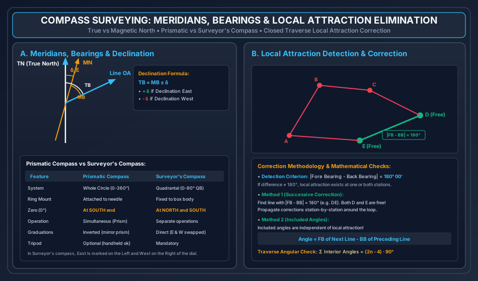
- East Declination (, positive): Magnetic North lies to the East of True North .
- West Declination (, negative): Magnetic North lies to the West of True North .
- Isogonic Lines: Lines joining geographic locations on the Earth's surface having identical magnetic declination.
- Agonic Line: The isogonic line connecting points of zero magnetic declination (, where Magnetic North coincides with True North).
2.4 Magnetic Dip () & The Aclinic Line
The magnetic dip is the vertical inclination angle that a freely suspended magnetic needle makes with the horizontal plane under the Earth's geomagnetic dipole field:
- At the Magnetic Equator: (horizontal needle). The line connecting points of zero dip is termed the Aclinic Line (Magnetic Equator).
- At the Magnetic Poles: (needle stands vertically).
- Counterpoise Rider: In the Northern Hemisphere, the North end of the needle dips downward; a small adjustable brass sliding weight (rider) is affixed to the South arm to restore horizontal equilibrium.
2.5 Closed Traverse Angular Geometry Check
For a closed polygon traverse with sides:
- Sum of Interior Angles:
- Sum of Exterior Angles:
- Included Angle at any Station: (If the computed value is negative, add . If the computed angle exceeds , it represents an exterior angle; the interior angle equals ).
3. Step-by-Step Analytical Derivations & Mechanisms
3.1 Independence of Included Angles from Local Attraction
Consider station connecting traverse lines and . Let station be affected by an unknown local magnetic disturbance causing an angular deflection error in the compass needle.
- Observed Fore Bearing of line :
- Observed Back Bearing of line (sighted from towards ):
- The included clockwise horizontal angle at station from line to line is:
- Substituting the error expressions:
- The local attraction error cancels out completely! Crucial Engineering Axiom: The horizontal angle between any two lines sighted from the same instrument station is entirely unaffected by local attraction at that station.
3.2 Mathematical Proof of Lehmann's Distance Proportionality Law
In the Three-Point Problem, let be three known ground control points plotted as on the plane table sheet. Let be the true ground position of the instrument, and let be its true plotted position on the sheet. Suppose the plane table board is accidentally mis-oriented by a small rotational angle (radians) about the plotted station .
- When the surveyor sights back through plotted point toward ground station , the actual line of sight on the mis-oriented sheet deviates from the true ray by angle .
- The perpendicular offset distance from the plotted ray to the true point on the sheet is:
- Similarly, for rays sighted toward stations and :
- Taking ratios:
- Since map distances are directly proportional to true ground distances by map scale : Lehmann's Second Rule: The perpendicular distance of the true station point from each of the three resection rays is strictly proportional to the actual distance of the corresponding ground station from the plane table.
3.3 The Danger Circle Condition (Indeterminate Resection)
Let be three control stations lying on the circumference of a circle (the Great Circumscribing Circle).
- By elementary circle geometry, the angle subtended by chord at any point on the circumference is constant: Similarly, chord subtends a constant angle:
- If the plane table is positioned at station on or very near this circumscribing circle:
- The angles and observed at will be satisfied by any point on the entire circular arc.
- When the table is oriented at any arbitrary, incorrect angle, the three resection rays drawn from will still intersect precisely at a single common point on the sheet!
- This single intersection gives a false, misleading illusion that the table is perfectly oriented and resection is complete, whereas the plotted point is completely bogus.
- Mathematically, the system of three resection equations becomes linearly dependent (determinant vanishes to zero).
- The Danger Circle Rule: Resection is geometrically indeterminate if the instrument station lies on or near the circle circumscribing the three reference stations. Field remedy: Select a fourth reference point or position the table well inside or outside the triangle.
4. Compass Instruments: Prismatic vs Surveyor's Compass
A precise understanding of the mechanical and optical distinctions between the two classic surveying compasses is essential for engineering practice.
            PRISMATIC COMPASS                      SURVEYOR'S COMPASS
      (Graduated Ring Moves with Needle)      (Needle Moves Independently Over Ring)
                     N                                      N (0°)
                     │                                      │
              W ─────┼───── E                        W ─────┼───── E
              (270°) │     (90°)                    (90°)   │    (90°)
                     S (0°)                                 S (0°)
           [Graduations Inverted;                 [East & West Swapped on Dial;
            Read Through Prism]                    Direct Eye Reading]
| Operational Characteristic | Prismatic Compass | Surveyor's Compass |
|---|---|---|
| Graduation Ring System | Whole Circle Bearing (WCB): clockwise. | Quadrantal Bearing (QB): Four quadrants . |
| Needle & Ring Construction | The broad magnetic needle is permanently attached to the lightweight aluminium graduated ring. The needle and ring rotate together as a single unit. | The graduated ring is rigidly attached to the brass box body; the edge-bar needle swings freely and independently on the pivot point. |
| Location of Zero () | Zero is engraved at the SOUTH end of the ring, at West, at North, and at East. | Zero is engraved at both NORTH and SOUTH ends; is engraved at East and West. |
| Orientation of Cardinal Points | Normal astronomical orientation (East on right, West on left). | East and West are swapped on the dial (East is marked on the Left and West on the Right) so that direct needle tip reading gives the correct quadrant. |
| Sighting & Reading Mechanism | Sighting the object vane and reading the graduated ring are performed simultaneously using an optical magnifying reflecting prism. | Sighting through the eye slit and reading the needle tip are performed as two separate operations from above the glass cover. |
| Optical Inversion | Graduations are engraved inverted (mirror writing) because they are viewed reflected through the hypotenuse prism. | Graduations are engraved upright and read directly by naked eye. |
| Tripod Requirement | Can be held in the hand or mounted on a light ball-and-socket tripod. | Cannot be used handheld; must be securely mounted on a sturdy tripod. |
5. Magnetic Declination, Dip & Secular/Diurnal Variations
5.1 Temporal Variations in Magnetic Declination
The Earth's geomagnetic field undergoes continuous temporal fluctuations:
- Secular Variation: A slow, progressive, wave-like swing in magnetic declination extending over cycles of (varying by several degrees). It is caused by convection currents of molten iron-nickel in the Earth's outer core.
- Annual Variation: A periodic seasonal swing varying by over a 12-month period.
- Diurnal Variation (Daily Variation): A 24-hour periodic oscillation caused by solar radiation ionizing the upper ionosphere:
- Amplitude: Varies from depending on geographic latitude.
- Higher in summer than in winter; higher near the poles than at the equator; greater during daylight hours than at night.
- Irregular Variation: Abrupt, sudden fluctuations of triggered by solar flares and magnetic geomagnetic storms.
6. Local Attraction: Detection, Source Identification & Elimination
6.1 Diagnostic Detection Criteria
At any survey station, local attraction is diagnosed by evaluating the absolute numerical difference between the forward and backward sightings along each line:
- If , both stations at the ends of that line are completely free from local attraction.
- If , local attraction exists at one or both stations.
6.2 Elimination Method 1: Method of Included Angles
- Compute the interior horizontal angle at every vertex:
- Sum the computed interior angles and verify against the theoretical geometric check:
- If a small observational closing discrepancy exists (), distribute it equally among all angles ().
- Identify a line that is entirely unaffected () to serve as the true starting datum.
- Derive all remaining forward and backward bearings sequentially using the corrected included angles.
6.3 Elimination Method 2: Method of Successive Corrections
- Identify the line whose . Both endpoints are certified free of local attraction.
- All bearings sighted from these unaffected stations are certified correct.
- The correct Back Bearing establishes the true Fore Bearing of the adjoining line by adding/subtracting .
- The error at the adjacent station equals:
- Apply this station correction to all other bearings observed from that station, and propagate the corrections sequentially around the traverse loop until closing.
7. Plane Table Surveying: Principles, Equipment & Essential Operations
7.1 Plane Table Equipment & Accessories
- Drawing Board: High-quality well-seasoned teak or pine board () mounted on a ball-and-socket leveling head tripod.
- Alidade:
- Plain Alidade: Straightedge brass/boxwood ruler with a beveled fiducial edge, carrying an eye-vane with a pinhole at one end and an object-vane with a vertical horsehair/cross-wire at the other.
- Telescopic Alidade: Optical telescope fitted with stadia hairs and vertical circle, enabling long-range sighting and simultaneous tacheometric distance/elevation determination.
- Plumbing Fork (U-Fork) with Plumb Bob: Used for precise Centering; transfers the plotted point on the drawing sheet directly over the ground station peg (or vice versa) within .
- Trough Compass: Long magnetic needle () housed in a rectangular brass box; used to mark the magnetic meridian along the edge of the drawing sheet.
- Spirit Level: Circular or tubular level used to ensure the board is strictly horizontal.
7.2 The Three Essential Operational Steps at Every Station
- Leveling: Squeezing the ball-and-socket head until the spirit level bubble remains centered in all positions.
- Centering: Aligning the plotted pin-point on paper vertically over ground peg using the plumbing fork and plumb bob.
- Orientation: Rotating the board in azimuth so that all lines on the paper become strictly parallel to their corresponding ground lines.
- Method A (By Magnetic Needle): Approximate; subject to local attraction errors.
- Method B (By Backsighting): High-precision; the alidade fiducial edge is aligned along line and the board is turned until station is bisected, clamping the board securely.
8. Plane Table Methods & The Two-Point / Three-Point Problems
8.1 The Four Classical Plane Table Methods
- Radiation: The plane table is set up at a central commanding station . Rays are drawn toward all detail features (), linear ground distances () are measured with a tape, and scaled off along the rays. Suitable for small open areas.
- Intersection (Graphic Triangulation): The locations of unknown points are plotted by the intersection of sighting rays drawn from the two endpoints of a measured baseline . No linear distance measurement to the target points is required! Ideal for inaccessible objects (river shores, steep hill peaks, marshy swamps).
- Traversing: The table is moved sequentially from station to station along a traverse loop (). At each station, the board is oriented by backsighting to the previous station and foresight rays are drawn to the forward station.
- Resection: The general process of locating the position of the plane table station on the drawing sheet using observations to pre-established ground stations.
8.2 Siting via the Three-Point Problem (Lehmann's Trial & Error Method)
When three visible control stations have their plotted positions on the drawing sheet:
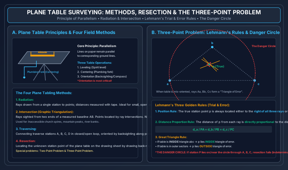
- Sighting to each station produces three rays that, if the board is mis-oriented, do not intersect at a single point, forming a Triangle of Error.
- Lehmann's Three Golden Rules locate the true position :
- Rule 1 (Position Rule): Point is located such that, facing the stations, it lies either to the right of all three rays or to the left of all three rays.
- Rule 2 (Proportional Distance Rule): The perpendicular distance from to each ray is proportional to the distance of the ground station from the table ().
- Rule 3 (Great Triangle Rule):
- If the table is set up INSIDE the great triangle , point lies INSIDE the triangle of error.
- If the table is set up in any of the six outer sectors, point lies OUTSIDE the triangle of error.
9. Embedded Technical Visualizations & Diagrams
9.1 Compass Meridians, Bearings & Local Attraction Elimination
The spatial geometry of True North, Magnetic North, magnetic declination, and the systematic elimination of local attraction around a closed polygon traverse are illustrated below.
9.2 Plane Table Surveying Methods & The Three-Point Problem
The four core plane tabling operations, alidade mechanics, the triangle of error, Lehmann's rules, and the Danger Circle condition are illustrated below.
10. Worked Analytical & Design Numerical Problems
Problem 1: Compass Closed Traverse Adjustment for Local Attraction
Statement: The following Fore and Back Bearings were recorded for a closed polygon traverse in an urban area where local magnetic disturbances were suspected:
| Line | Fore Bearing (FB) | Back Bearing (BB) |
|---|---|---|
- Detect the stations affected by local attraction.
- Determine the correct Fore and Back Bearings for all lines using the Method of Successive Corrections.
- Verify the traverse geometry using the Included Angles Method and confirm the theoretical sum .
Analytical Solution:
Step 1: Diagnostic Check of Bearing Differences ()
- Line : (Affected)
- Line : (Affected)
- Line : (Affected)
- Line : Stations and are completely FREE from local attraction!
- Line : (Affected)
Step 2: Successive Correction Propagation from Unaffected Stations &
- Line : Both and are free:
- Line : Observed at , so is correct:
- Observed .
- Error at Station .
- .
- Line : Observed Back Bearing sighted from :
- .
- .
- .
- Observed .
- Error at Station .
- .
- Line : Observed Back Bearing sighted from :
- .
- .
- .
- Observed .
- Error at Station .
- .
- Check on Line : Station is certified free:
- .
- .
- Observed at Station .
- Applying correction at Station ():
Corrected Bearings Summary Table:
| Line | Correct Fore Bearing (FB) | Correct Back Bearing (BB) |
|---|---|---|
Step 3: Verification via Included Angles Method Formula: :
Sum of interior angles:
Problem 2: Magnetic Declination, True Bearings & Secular Epoch Shifts
Statement: In the year 1990, the magnetic bearing of a boundary property line was recorded with a surveyor's compass as . The Survey of India magnetic record shows that the magnetic declination at the location in 1990 was . In the year 2026, the magnetic declination at the same station is measured to be . Calculate:
- The True Bearing of line .
- The current Magnetic Bearing of line in the year 2026 in both Whole Circle Bearing and Quadrantal Bearing systems.
Analytical Solution:
Step 1: True Bearing Determination (From 1990 Data) Given:
- .
- Magnetic Declination in 1990: .
(Note: The True Bearing is fixed to the geographical pole and remains permanently constant over centuries).
Step 2: Magnetic Bearing in Year 2026 Given:
- Declination in 2026: .
In Quadrantal Bearing format:
Problem 3: Three-Point Problem Lehmann's Ray Offset Analysis
Statement: In a plane table survey, three control stations are plotted on the drawing sheet as . An instrument setup at unknown ground station produces a triangle of error with ray offsets. The ground distances from the plane table to the reference stations are measured by rangefinder as:
If the perpendicular distance of the true plotted station from ray is determined to be on the sheet, compute:
- The exact perpendicular offset distances and from rays and to the true point on the sheet.
- State the relative spatial side constraint (left vs right) that point must satisfy relative to the three sight rays.
Analytical Solution:
Step 1: Application of Lehmann's Second Rule (Distance Proportionality) Per Lehmann's law:
Given and :
Computing and :
Step 2: Position Orientation Rule By Lehmann's First Rule, facing each reference station in turn:
11. Cross-Exam Synthesis Matrix
| Exam | High-Frequency Conceptual Focus | Typical Calculation Types | Priority Traps & Critical Nuances |
|---|---|---|---|
| GATE CE | • Local attraction detection and correction • Included angles from bearings • Declination conversion () • Three-Point Problem Danger Circle |
• Numerical Answer Type (NAT) corrected bearings • Angle between lines from bearings • Shift in magnetic bearing over time |
• When , BOTH stations are free from local attraction! • In , East is POSITIVE and West is NEGATIVE in WCB. • If computed angle is negative, add . |
| UPSC ESE | • Full derivation of Lehmann's rules • Two-Point vs Three-Point problem methods • Surveyor's vs Prismatic compass dial construction • Aclinic line, Isogonic/Agonic lines |
• Conventional 15-mark closed traverse adjustment • Bessel's graphical solution for 3-point resection • Dip and declination variations |
• In Surveyor's compass, East is on the LEFT of the dial and West is on the RIGHT! • Zero is at the SOUTH in Prismatic compass ring. • Danger circle occurs when station lies on circumscribing circle of . |
| SSC JE / RRB JE | • Graduation positions on Prismatic ( at South) vs Surveyor's ( at N & S) • Fore bearing to Back bearing conversion () • Plane table accessories (Plumbing fork, Alidade, Trough compass) • Orientation by backsighting |
• Quick WCB to QB conversions • Back bearing computation • Traverse angle sum |
• In QB system, Back Bearing has the EXACT SAME numerical value, only quadrant letters reverse! • Centering is done with plumbing fork; leveling with spirit level; orientation by backsighting. • Alidade has a beveled edge termed the fiducial edge. |
| State AE / PSU | • Methods of plane tabling (Radiation, Intersection, Traversing, Resection) • Resection definition • Inaccessible points solved by Intersection • Dip value at equator () and poles () |
• Corrected bearing calculation with local attraction • Declination algebraic addition • Error propagation in traverse |
• Intersection method requires NO linear distance measurement to details! • Dip is at magnetic equator; at magnetic poles. • Most accurate method of plane table orientation is backsighting. |
12. Common Failure Modes, Magnetic Distortion Diagnostics & Forensic Engineering
12.1 Undetected Local Attraction from Buried Utilities
- Failure Phenomenon: A boundary retracement survey executed with a compass establishes misaligned property lines that encroach several metres into adjacent plots, sparking legal litigation.
- Root Cause & Forensic Diagnosis:
- The surveyor set up the compass over an innocent-looking grass verge beneath which a ductile iron water main ( dia) and a high-voltage buried power cable were running.
- The magnetic needle suffered a continuous, undetected deflection.
- Forensic Countermeasures:
- Always verify on every traverse line without exception.
- Sighting with an optical theodolite or electronic total station completely immune to magnetic disturbance.
12.2 Plane Table Mis-Orientation from Loose Clamp
- Failure Phenomenon: During a multi-hour mapping session, plotted points progressively shear away from their true ground topography.
- Root Cause: The wing-nut clamping screw under the ball-and-socket head was improperly torqued, allowing the table board to rotate slightly every time the surveyor leaned against the board to sight the alidade.
- Site Rule: Never apply body weight to the table; re-verify orientation by sighting a distant reference mark after plotting every 5 details.
13. Practice Problems & Exam Drill Questions
Question 1 (GATE Style — NAT)
The magnetic bearing of a line was observed to be . If the magnetic declination at that station is , determine the true bearing of line in the Whole Circle Bearing (WCB) system in degrees. (Express to two decimal places).
- Answer:
- Explanation:
- In WCB, corresponds to: .
- Declination is .
- .
Question 2 (UPSC ESE Style — Conceptual Multiple Choice)
Which of the following statements regarding Compass and Plane Table Surveying is/are CORRECT?
- In a surveyor's compass, the graduated ring is fixed to the box and East and West are reversed.
- In plane table surveying, orientation by backsighting is more reliable than orientation by trough compass.
- The Three-Point Problem becomes indeterminate if the instrument station lies on the circle circumscribing the three control stations.
- Local attraction affects the included angle computed between two lines sighted from the affected station.
- Options: (a) 1, 2, and 3 only (b) 1, 3, and 4 only (c) 2 and 4 only (d) 1, 2, 3, and 4
- Correct Answer: (a) 1, 2, and 3 only
- Explanation: Statement 4 is incorrect because local attraction error affects both lines equally and cancels out completely in subtraction; included angles are strictly independent of local attraction. Statements 1, 2, and 3 are entirely correct.
Question 3 (SSC JE / RRB JE Style — Quick Recall)
The horizontal angle between the true meridian and the magnetic meridian at a place is known as:
- Options: (a) Magnetic Dip (b) Magnetic Declination (c) Local Attraction (d) Bearing
- Correct Answer: (b) Magnetic Declination
- Explanation: Magnetic declination is the horizontal angle between the True Meridian and the Magnetic Meridian. Magnetic dip is the vertical inclination of the needle with the horizontal.
14. Comprehensive Technical Reference & Cross-Topic Linkages
Inter-Topic Knowledge Mapping
- Upstream Linkages:
SURV-01: Fundamental surveying principles (Working from whole to part, error types).
- Concurrent & Downstream Linkages:
SURV-03: Levelling, reciprocal sights, and line of collimation errors.SURV-04: Theodolite traversing, coordinate geometry (latitudes and departures), Bowditch traverse balancing.SURV-06: Total stations, electronic compasses, GNSS heading determination.
Standard Code References
- IS 1492 / IS 1957: Specification for Surveying Prismatic Compasses.
- IS 2533: Specification for Plane Tables and Accessories, Bureau of Indian Standards.
- Survey of India: Topographical Surveying Manual, Dehradun.