Municipal Solid Waste Management, Air Pollution & Noise Pollution
In this chapter (1 topics)
On this page
- 1. Topic Title & Authoritative References
- 2. Prerequisites & Learning Objectives
- Prerequisites
- Learning Objectives
- 3. Municipal Solid Waste (MSW) Engineering & Characterization
- 3.1 Physical & Chemical Characterization
- 3.2 Composite Density & Moisture Formulations
- 4. Solid Waste Processing, Composting & Thermal Conversion
- 4.1 Composting of Organic Waste
- 4.2 Thermal Conversion Technologies
- 5. Engineered Sanitary Landfills (SWM Rules 2016)
- 5.1 Landfill Cell Operation
- 5.2 Multi-Barrier Bottom Liner System (SWM Rules 2016 Standards)
- 5.3 Landfill Gas (LFG) Recovery
- 6. Air Pollution Meteorology, Stability & Plume Dispersion
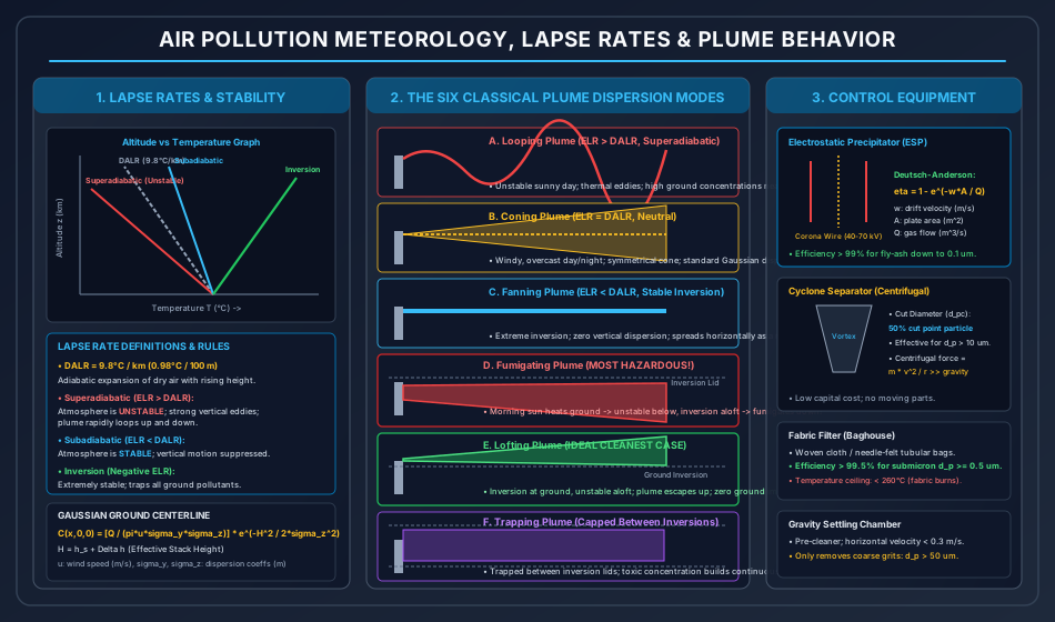
- 6.1 Atmospheric Lapse Rates & Stability
- 6.2 The Six Classical Plume Dispersion Behaviors
- 6.3 Effective Stack Height (H)
- 6.4 Gaussian Plume Dispersion Model
- 7. Particulate & Gaseous Air Pollution Control Devices
- 7.1 Particulate Matter Control Equipment
- 7.2 Gaseous Pollutant Control
- 8. Noise Pollution Engineering & Regulatory Standards
- 8.1 Acoustic Decibel Definitions
- 8.2 Addition of Non-Coherent Sound Levels
- 8.3 Statistical & Equivalent Noise Descriptors
- 8.4 CPCB Noise Regulation Rules (2000) Statutory Limits
- 9. Step-by-Step Analytical Derivations
- 9.1 Derivation of Composite Solid Waste Density Formula
- 9.2 Derivation of Ground-Level Centerline Gaussian Dispersion Equation
- 9.3 Derivation of Deutsch-Anderson ESP Efficiency Equation
- 10. Solved Numerical Example 1: MSW Density, Energy & Landfill Sizing
- Problem Statement
- Complete Analytical Solution
- 11. Solved Numerical Example 2: Gaussian Plume Dispersion & ESP Sizing
- Problem Statement
- Complete Analytical Solution
- 12. Solved Numerical Example 3: Noise Decibel Addition & Day-Night Level
- Problem Statement
- Complete Analytical Solution
- 13. Common Misconceptions & Exam Traps
- 14. Quick Revision Summary & Formula Sheet
- 14.1 Governing Mathematical Formulas
- 14.2 High-Yield Exam Memorization Matrix
1. Topic Title & Authoritative References
Title: Municipal Solid Waste Engineering (Characterization, Proximate/Ultimate Analysis, Composting, Incineration, Sanitary Landfill Multi-Barrier Liners per SWM Rules 2016), Atmospheric Meteorology & Plume Dynamics, Gaussian Dispersion Modeling, Air Pollution Control Equipment (ESP, Cyclones, Baghouses, Scrubbers), and Environmental Noise Pollution (Decibel Physics, , CPCB Noise Rules 2000).
Primary Standards & Authoritative Specifications:
- CPHEEO Manual (2016 / 2024 draft): Manual on Municipal Solid Waste Management (Part I: Management; Part II: Engineering; Part III: Compendium), Ministry of Housing and Urban Affairs, Government of India.
- Solid Waste Management (SWM) Rules, 2016: Ministry of Environment, Forest and Climate Change (MoEFCC), Government of India.
- NAAQS (2009): National Ambient Air Quality Standards, Central Pollution Control Board (CPCB), Notification No. B-29016/20/90/PCI-L.
- Noise Pollution (Regulation and Control) Rules, 2000: MoEFCC, Government of India.
- IS 10037 / IS 10440: Codes of Practice for Solid and Hazardous Waste Management.
- Wark, K., Warner, C. F., & Davis, W. T. (1998): Air Pollution: Its Origin and Control (3rd Edition), Prentice Hall.
- Tchobanoglous, G., Theisen, H., & Vigil, S. A. (1993): Integrated Solid Waste Management: Engineering Principles and Management Issues, McGraw-Hill.
2. Prerequisites & Learning Objectives
Prerequisites
- Atmospheric physics: Hydrostatic equation, dry adiabatic expansion (), buoyancy forces, thermal eddy turbulence.
- Chemical thermodynamics: Combustion stoichiometry, Dulong's calorific equation, carbon-to-nitrogen ratios, gas laws ().
- Acoustics & logarithmic mathematics: Wave mechanics, sound pressure (), acoustic intensity (), decibel logarithmic transformations.
Learning Objectives
- Perform proximate and ultimate analyses of municipal solid waste (MSW), and calculate composite density, composite moisture content, and energy heating values.
- Formulate biological and thermal waste conversion processes, distinguishing between Indore (aerobic) and Bangalore (anaerobic) composting, optimizing C/N ratios (), and applying the principles of incineration.
- Detail multi-barrier engineered sanitary landfills under SWM Rules 2016, specifying compacted clay liner thickness (), HDPE geomembrane barriers (), and leachate collection and removal systems (LCRS).
- Evaluate atmospheric stability using Environmental Lapse Rates (ELR) and Dry Adiabatic Lapse Rates (DALR), diagnosing the six classical plume dispersion behaviors (Looping, Coning, Fanning, Fumigating, Lofting, Trapping).
- Apply the Gaussian plume dispersion model to compute ground-level centerline pollutant concentrations downstream of industrial stacks.
- Design air pollution particulate control devices, applying the Deutsch-Anderson equation for Electrostatic Precipitators (ESP) and cut-diameter equations for cyclone separators.
- Solve acoustic noise problems, adding non-coherent decibel sources, computing equivalent continuous sound levels () and Day-Night levels (), and verifying compliance with CPCB Noise Rules 2000.
3. Municipal Solid Waste (MSW) Engineering & Characterization
3.1 Physical & Chemical Characterization
Solid waste from domestic, commercial, and institutional establishments comprises biodegradable organic food waste, combustible paper/plastics, and inert mineral matter.
1. Proximate Analysis
Determines combustible characteristics of solid waste through sequential heating:
- Moisture Content (): Loss in weight upon drying at for .
- Volatile Combustible Matter (VCM): Additional loss in weight upon heating at in a closed crucible without oxygen.
- Fixed Carbon (FC): Combustible residue remaining after volatile expulsion.
- Ash: Non-combustible inorganic mineral residue remaining after ignition at with open oxygen.
2. Ultimate Analysis
Quantifies elementary chemical percentages by weight: Carbon (), Hydrogen (), Oxygen (), Nitrogen (), Sulfur (), and non-combustible Ash.
3. Energy Heating Value (Dulong's Formula)
The higher heating value (HHV) in on as-discarded dry basis:
Where are percentage masses of carbon, hydrogen, oxygen, and sulfur.
3.2 Composite Density & Moisture Formulations
Because solid waste is a heterogeneous multi-component aggregate:
- Composite As-Discarded Density ():
Where is the mass percentage and is the loose density of component ().
- Typical loose uncompacted density: (Western nations) to (Indian cities due to high ash, organic, and moisture content).
- Composite Moisture Content ():
4. Solid Waste Processing, Composting & Thermal Conversion
4.1 Composting of Organic Waste
Biological decomposition of putrescible organic waste by mixed microbial cultures into stable humic compost.
- Aerobic Composting:
- Thermophilic temperatures () destroy weed seeds and pathogens.
- Indore Method: Developed by Howard and Wad; strictly aerobic method conducted in open piles or trenches with manual or mechanical turning at 16, 30, and 60 days; stabilizes compost in .
- Windrow Composting: Long trapezoidal piles ( height, base) turned mechanically once or twice weekly.
- Anaerobic Composting:
- Bangalore Method: Developed by Dr. C. N. Acharya; conducted in earthen pits covered with mud plaster; operates under anaerobic conditions without turning; slower decomposition (), but eliminates odor and nutrient volatilization.
- Critical Composting Control Parameters:
- Carbon-to-Nitrogen Ratio (C/N Ratio):
- Optimum range:
- If : Nitrogen becomes growth-limiting; decomposition slows drastically.
- If : Excess nitrogen volatilizes as foul ammonia gas ().
- Moisture Content: Optimum (below , microbial activity ceases; above , water fills pore voids triggering anaerobic odors).
- Carbon-to-Nitrogen Ratio (C/N Ratio):
4.2 Thermal Conversion Technologies
- Incineration: Controlled high-temperature combustion of waste in excess oxygen ():
- The Rule: High Temperature ( to crack dioxins/furans), Adequate Residence Time ( in secondary chamber), High Turbulence (excess air ).
- Reduces waste volume by and mass by .
- Pyrolysis: Thermal degradation in the total absence of oxygen (), producing bio-char, bio-oil, and syngas.
- Gasification: Thermal conversion under substoichiometric oxygen (), generating synthesis gas ().
5. Engineered Sanitary Landfills (SWM Rules 2016)
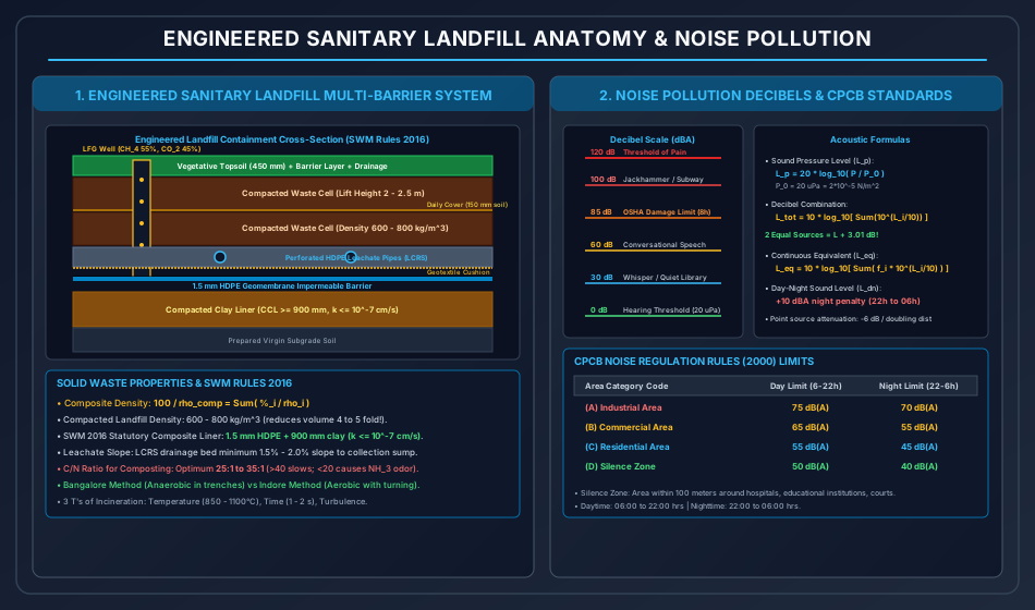
Sanitary landfilling is the controlled biological stabilization of non-recyclable and non-compostable municipal waste on land without creating nuisance or environmental hazards to groundwater and public health.
5.1 Landfill Cell Operation
- Daily Cell: Waste deposited in layers (), compacted by heavy wheeled landfill compactors () to achieve compacted density .
- Daily Soil Cover: Covered at the end of each working day with () of compacted soil to prevent bird scavenging, fly breeding, windblown litter, and odor.
- Intermediate Cover: Layer of placed over completed cell lifts left exposed for .
- Lift Height: Each waste lift is typically .
5.2 Multi-Barrier Bottom Liner System (SWM Rules 2016 Standards)
To provide absolute protection against leachate percolation into aquifers:
- Compacted Clay Liner (CCL) / Low Permeability Soil:
- Minimum thickness: ().
- Saturated hydraulic conductivity: ().
- Flexible Synthetic Membrane Barrier (Geomembrane):
- High Density Polyethylene (HDPE) smooth or textured geomembrane.
- Minimum thickness: .
- Geotextile Protection Cushion:
- Non-woven needle-punched geotextile () placed over geomembrane to prevent puncturing by drainage aggregate.
- Leachate Collection & Removal System (LCRS):
- Granular drainage blanket of washed rounded gravel: minimum thickness , permeability .
- Perforated corrugated HDPE pipes (minimum diameter ) laid at a minimum longitudinal slope of , directing leachate to an external sump for chemical/biological treatment.
5.3 Landfill Gas (LFG) Recovery
Anaerobic degradation inside mature landfill cells generates landfill gas:
- Composition: (methane), , trace non-methane organic compounds (NMOCs).
- Hazard: Methane is explosive when mixed with air in the concentration range of by volume (Lower Explosive Limit LEL , Upper Explosive Limit UEL ).
- Vertical perforated extraction wells connected to vacuum blowers recover LFG for electrical generation.
6. Air Pollution Meteorology, Stability & Plume Dispersion
6.1 Atmospheric Lapse Rates & Stability
The vertical temperature gradient of the ambient troposphere controls whether atmospheric turbulence suppresses or amplifies vertical plume dispersion.
- Dry Adiabatic Lapse Rate (DALR, ): The theoretical rate of temperature decrease experienced by a dry, unconfined parcel of air rising adiabatically:
- Environmental Lapse Rate (ELR, ): The actual measured ambient temperature decrease with altitude:
Atmospheric Stability Regimes
- Superadiabatic (): Ambient temperature drops faster than . Rising parcels are warmer than surrounding air Highly buoyant UNSTABLE ATMOSPHERE.
- Neutral (): Parcel temperature matches ambient NEUTRAL STABILITY.
- Subadiabatic (): Temperature drop is less than STABLE ATMOSPHERE.
- Isothermal (): Temperature constant with altitude HIGHLY STABLE.
- Inversion (, Negative Lapse Rate): Temperature increases with altitude EXTREME STABILITY; traps pollutants at ground level.
6.2 The Six Classical Plume Dispersion Behaviors
| Plume Behavior | Ambient Lapse Rate Condition | Visual Dispersion Pattern | Ground-Level Pollution Hazard |
|---|---|---|---|
| 1. Looping Plume | Superadiabatic () Unstable atmosphere with high solar heating. |
Rapidly loops up and down in large rolling thermal eddies. | High intermittent ground-level concentrations close to the stack. |
| 2. Coning Plume | Neutral () Windy, cloudy days or overcast nights. |
Symmetrical cone spreading outward along the centerline. | Moderate, predictable ground concentrations far from stack. |
| 3. Fanning Plume | Strong Surface Inversion () Stable night atmosphere. |
Thin horizontal ribbon with zero vertical dispersion; spreads horizontally. | Zero ground contact; harmless until morning sunrise. |
| 4. Fumigating Plume | Inversion Aloft + Superadiabatic Below Morning sun heats ground, breaking surface inversion. |
Bottom of plume plunges downwards rapidly, blocked by inversion aloft. | MOST DANGEROUS TOXIC SPIKE: Extremely high ground concentrations! |
| 5. Lofting Plume | Surface Inversion + Superadiabatic Aloft Late afternoon / sunset. |
Plume spreads freely upward into unstable air; zero downward mixing. | IDEAL CLEANEST CASE: Zero pollutant reaching ground. |
| 6. Trapping Plume | Inversion Layers Both Above and Below Stack | Plume trapped completely between upper and lower inversion lids. | High continuous accumulation within the bounded atmospheric layer. |
6.3 Effective Stack Height ()
The physical stack height () plus the buoyant/momentum plume rise ():
Holland's Plume Rise Equation:
Where is stack exit velocity (), is stack inside diameter (), is wind speed (), is atmospheric pressure (), and are stack gas and ambient temperatures ().
6.4 Gaussian Plume Dispersion Model
For a continuous point source emitting pollutant at rate () at effective height with mean wind speed ():
Ground-Level Centerline Concentration ():
Where are Pasquill-Gifford dispersion coefficients () growing with downwind distance .
7. Particulate & Gaseous Air Pollution Control Devices
7.1 Particulate Matter Control Equipment
- Gravity Settling Chambers: Large horizontal expansion chambers (); removes coarse grit .
- Cyclone Separators: Dirty gas enters tangentially at velocity , creating a high-speed vortex where centrifugal acceleration () flings particles against the outer walls.
- Cut Diameter (): Particle size collected with exactly efficiency: Where is cyclone inlet width, is effective number of turns (), and is dynamic gas viscosity.
- Fabric Filters (Baghouses): Tubular fabric bags (woven or needle-punched felt); gas flows through fabric leaving a dust cake; high efficiency () down to . Temperature ceiling: (Teflon/fiberglass).
- Electrostatic Precipitators (ESP):
- High voltage DC negative corona () ionizes flue gas; negative gas ions charge dust particles; particles migrate to grounded positive collecting plates.
- Deutsch-Anderson Efficiency Equation: Where is particle drift migration velocity (), is total collecting plate area (), and is flue gas volumetric discharge ().
7.2 Gaseous Pollutant Control
- Flue Gas Desulfurization (FGD): Wet limestone scrubbers remove ().
- Selective Catalytic Reduction (SCR): Injects ammonia () over titanium oxide catalysts at to reduce to benign and .
8. Noise Pollution Engineering & Regulatory Standards
Sound represents mechanical pressure oscillations propagating through an elastic medium. Because the human ear responds logarithmically across a massive acoustic pressure dynamic range ( to ), noise is quantified on a decibel () scale.
8.1 Acoustic Decibel Definitions
- Sound Pressure Level (): Where (the standard threshold of human hearing at ).
- Sound Power Level (): Where reference sound power .
- Sound Intensity Level (): Where reference sound intensity .
8.2 Addition of Non-Coherent Sound Levels
Sound pressure levels cannot be summed linearly! Pressures must be converted to energy intensities:
Two Equal Sound Sources Rule:
If two identical sources each producing operate simultaneously:
8.3 Statistical & Equivalent Noise Descriptors
- Equivalent Continuous Sound Level (): The steady-state A-weighted sound level that transmits the identical acoustic energy over a specified time interval : Where is the fraction of total time spent at sound level .
- Day-Night Average Sound Level (): Integrates noise over 24 hours, imposing a severe weighting penalty on nighttime noise () to account for sleep disturbance:
- Statistical Exceedance Levels:
- : Sound level exceeded for of measurement duration (represents peak road traffic noise).
- : Sound level exceeded for of time (median noise level).
- : Sound level exceeded for of time (ambient background noise).
8.4 CPCB Noise Regulation Rules (2000) Statutory Limits
Ambient air quality standards in respect of noise:
| Area Category Code | Category of Area / Zone | Day Time Limits () | Night Time Limits () |
|---|---|---|---|
| (A) | Industrial Area | ||
| (B) | Commercial Area | ||
| (C) | Residential Area | ||
| (D) | Silence Zone |
Statutory Definition of Silence Zone: An area comprising not less than around hospitals, educational institutions, courts, and religious shrines declared by competent authority.
9. Step-by-Step Analytical Derivations
9.1 Derivation of Composite Solid Waste Density Formula
Consider a composite solid waste batch of total mass composed of distinct physical waste components with mass fractions (where ) and uncompacted densities .
The mass of individual component is:
The volume occupied by individual component () is:
Assuming no volume contraction upon initial mixing, the total composite uncompacted volume () is:
By definition, the composite density of the mixture () is:
Expressing mass fractions as percentages :
9.2 Derivation of Ground-Level Centerline Gaussian Dispersion Equation
The 3D Gaussian plume equation for a steady-state elevated release at effective height with perfect ground reflection () is:
For a ground-level receptor directly along the downwind centerline axis:
Substitute into the vertical reflection bracket:
Substitute Eq. (2) and Eq. (4) into Eq. (1):
Canceling the factor of :
9.3 Derivation of Deutsch-Anderson ESP Efficiency Equation
Consider a horizontal flue gas flow through an Electrostatic Precipitator channel of cross-sectional area , width , height , and length . The gas flows at volumetric rate with mean velocity .
Let be the constant electrostatic drift migration velocity of charged dust particles toward the parallel collecting plates.
Consider a differential control slice of length along the gas flow direction.
The gas transit time across this differential length is .
During time , particles within a distance from the collecting plate strike the plate and are captured.
The fraction of particles captured across differential slice is:
Where is the differential collecting plate surface area.
Integrating along the entire length of the precipitator from inlet () to outlet ():
Taking the exponential on both sides:
The collection efficiency is the fraction of particles removed:
Substituting Eq. (4) into Eq. (5):
10. Solved Numerical Example 1: MSW Density, Energy & Landfill Sizing
Problem Statement
An urban municipality with a population of generates municipal solid waste at a per-capita rate of .
The physical and chemical composition of the as-discarded solid waste is tabulated below:
| Waste Component | Weight Fraction () | Loose Density (, ) | Moisture Content (, ) | Energy Content (, ) |
|---|---|---|---|---|
| Food Waste | ||||
| Paper | ||||
| Plastics | ||||
| Cardboard | ||||
| Yard Waste | ||||
| Glass & Inerts |
- Calculate the total daily MSW generation in .
- Determine the composite as-discarded density ( in ).
- Compute the composite moisture content () and average energy content on as-discarded basis ().
- If this waste is compacted in an engineered sanitary landfill to a density of with daily soil cover accounting for of the total landfill volume, determine the total annual landfill volume required () and the landfill footprint area in hectares for a total compacted lift height of .
Complete Analytical Solution
1. Total Daily MSW Generation
2. Composite Density ()
3. Composite Moisture & Energy Content
- Composite Moisture:
- Average Energy Content:
4. Landfill Volume & Footprint Sizing
Accounting for soil cover volume ():
For a total compacted lift height of :
11. Solved Numerical Example 2: Gaussian Plume Dispersion & ESP Sizing
Problem Statement
A coal-fired power station emits sulfur dioxide () gas at a steady continuous rate of from a physical stack of height .
The thermal buoyancy and momentum plume rise is , yielding an effective stack height of .
The average wind speed at stack height is .
At a downwind receptor location directly along the plume centerline, the atmospheric dispersion coefficients are and .
- Calculate the ground-level centerline concentration () in micrograms per cubic meter ().
- An Electrostatic Precipitator (ESP) treats a flue gas flow of . If the migration drift velocity of fly-ash particles is , calculate the collecting plate area () required to achieve a collection efficiency of via the Deutsch-Anderson equation.
Complete Analytical Solution
1. Ground-Level Centerline Concentration
Using the Gaussian ground-level centerline formula:
Given:
Compute the denominator:
Compute the exponential argument:
Calculate concentration:
2. Electrostatic Precipitator Plate Sizing
Using the Deutsch-Anderson equation:
Taking the natural logarithm:
Given and :
12. Solved Numerical Example 3: Noise Decibel Addition & Day-Night Level
Problem Statement
- In an industrial machine shop, four independent fabrication machines operate concurrently, producing individual sound pressure levels of , , , and .
- (a) Calculate the total combined sound pressure level in the workshop.
- (b) If Machine 3 () is turned off, determine the new combined noise level and the net noise reduction achieved.
- A 24-hour environmental noise monitoring survey conducted in a residential zone yielded the following hourly sound pressure levels:
- Daytime (, duration ):
- Evening (, duration ):
- Nighttime (, duration ): Calculate the 24-hour equivalent continuous sound level () and the Day-Night Average Sound Level ().
Complete Analytical Solution
1. Machine Shop Decibel Combination
-
(a) All Four Machines Operating:
-
(b) Without Machine 3 ():
2. Environmental and
-
(a) 24-Hour Equivalent Continuous Sound Level ():
-
(b) Day-Night Average Sound Level (): Nighttime period () carries penalty :
13. Common Misconceptions & Exam Traps
[!WARNING] Trap 1: Looping vs Fumigating Plumes
Candidates frequently confuse the ground pollution hazard of looping vs fumigating:
- Looping: Occurs during bright sunny afternoons under superadiabatic conditions (). The plume loops up and down; ground contacts are patchy and intermittent.
- Fumigating: Occurs shortly after sunrise when morning solar radiation heats the ground, creating an unstable layer beneath a persistent radiation inversion lid. The plume is completely prevented from rising and is forced straight down to the ground, creating the highest, most lethal ground-level concentrations.
[!WARNING] Trap 2: Adding Decibels Linearly
A classic blunder in competitive exams: "If two machines each produce , what is the total sound level?" Candidates frequently answer .
In reality, is the threshold of pain ( more energetic!). The correct answer is:
[!CAUTION] Trap 3: SWM 2016 Liner Composite Structure
In UPSC/GATE questions regarding engineered landfill liners, note the dual-barrier mandate:
- Minimum HDPE geomembrane
- Overlying compacted clay liner with .
Providing clay alone or geomembrane alone does NOT satisfy modern statutory environmental regulations!
[!IMPORTANT] Trap 4: C/N Ratio Thresholds in Composting
The optimum C/N ratio is (conventionally remembered as ).
- If , micro-organisms starve for nitrogen, and the process stalls.
- If , excess nitrogen cannot be incorporated into cell protein and volatilizes as odorous ammonia ().
[!NOTE] Trap 5: Nighttime Penalty in
In computing , the penalty is added directly to the measured nighttime decibel level before energy averaging (). Candidates often mistakenly add to the final 24-hour average, yielding an incorrect result.
14. Quick Revision Summary & Formula Sheet
14.1 Governing Mathematical Formulas
- Composite Solid Waste Density:
- Dulong's Higher Heating Value:
- Gaussian Centerline Ground Concentration:
- Deutsch-Anderson ESP Efficiency:
- Sound Pressure Level:
- Decibel Combination (Energy Sum):
- Equivalent Continuous Sound Level ():
- Day-Night Average Level ():
14.2 High-Yield Exam Memorization Matrix
| Feature / Standard | Statutory Value / Design Requirement |
|---|---|
| DALR | (). |
| Most Dangerous Plume | Fumigating Plume (ground inversion heats from below, capped by inversion aloft). |
| Cleanest Plume | Lofting Plume (surface inversion, superadiabatic aloft; zero ground contact). |
| Composting C/N Ratio | Optimum (Indore is aerobic; Bangalore is anaerobic). |
| Landfill Liner (SWM 2016) | clay () HDPE geomembrane. |
| Landfill Gas Composition | , (Explosive range ). |
| CPCB Noise - Residential | Day (), Night (). |
| CPCB Noise - Silence Zone | Day, Night ( radius around hospitals/schools). |
| ESP Application | High voltage (); removes submicron fly-ash with efficiency. |
| Acoustic Reference | . |