ENV-06 Chapter 06 · Sludge Treatment and Disposal

Sludge Treatment & Stream Effluent Disposal (Streeter-Phelps DO Sag Analysis)

In this chapter (1 topics)
On this page
  1. 1. Topic Title & Authoritative References
  2. 2. Prerequisites & Learning Objectives
  3. Prerequisites
  4. Learning Objectives
  5. 3. Sludge Generation, Characterization & Volume-Moisture Relations
  6. 3.1 Sources & Types of Wastewater Sludge
  7. 3.2 Specific Gravity of Sludge & Solids
  8. 3.3 The Sludge Volume-Moisture Relationship
  9. 4. Sludge Thickening & Conditioning
  10. 4.1 Sludge Thickening Processes
  11. 4.2 Sludge Conditioning
  12. 5. Anaerobic Sludge Digestion Engineering
  13. 5.1 Environmental Operating Regimes
  14. 5.2 Reactor Configurations: Standard-Rate vs High-Rate
  15. 5.3 Digester Capacity Formulation
  16. 5.4 Biogas Energy Yield
  17. 6. Sludge Dewatering & Final Disposal
  18. 7. River Stream Self-Purification & Ecological Zones
  19. 7.1 Hydrodynamic Initial Mix at Outfall
  20. 7.2 The Four Ecological Zones of Stream Self-Purification
  21. 8. The Streeter-Phelps Dissolved Oxygen Sag Formulation
  22. 8.1 The Governing Differential Equation
  23. 8.2 Integrated Streeter-Phelps Equation
  24. 8.3 Critical DO Sag Point: Time (tc) & Deficit (Dc)
  25. 9. Step-by-Step Analytical Derivations
  26. 9.1 Derivation of Sludge Volume-Moisture Equation
  27. 9.2 Derivation of Streeter-Phelps Integrated Deficit Equation
  28. 9.3 Derivation of Critical Time (tc) and Critical Deficit (Dc)
  29. 10. Solved Numerical Example 1: Sludge Thickening, Dewatering & S.G.
  30. Problem Statement
  31. Complete Analytical Solution
  32. 11. Solved Numerical Example 2: Anaerobic Digester Sizing & Biogas Generation
  33. Problem Statement
  34. Complete Analytical Solution
  35. 12. Solved Numerical Example 3: Streeter-Phelps River DO Sag Analysis
  36. Problem Statement
  37. Complete Analytical Solution
  38. 13. Common Misconceptions & Exam Traps
  39. 14. Quick Revision Summary & Formula Sheet
  40. 14.1 Governing Mathematical Formulas
  41. 14.2 High-Yield Exam Memorization Matrix

1. Topic Title & Authoritative References

Title: Sludge Generation, Volume-Moisture Kinetics, Gravity Thickening, Anaerobic Sludge Digestion (Mesophilic vs Thermophilic, Digester Sizing, Biogas Energy Recovery), Sludge Conditioning & Dewatering, River Stream Self-Purification Ecology, and the Streeter-Phelps Dissolved Oxygen (DO) Sag Model.
Primary Standards & Authoritative Specifications:

  • CPHEEO Manual (2013 / 2024 update): Manual on Sewerage and Sewage Treatment Systems (Part A: Engineering; Part B: O&M), Ministry of Housing and Urban Affairs, Government of India.
  • IS 10037 (Parts 1 to 3): Requirements for Sludge Dewatering Equipment: Sludge Drying Beds, Rotary Drum Vacuum Filters, Centrifuges.
  • CPCB Environmental Standards: General Standards for Discharge of Environmental Pollutants — Part A: Effluents, Central Pollution Control Board, Government of India.
  • Streeter, H. W., & Phelps, E. B. (1925): A Study of the Pollution and Natural Purification of the Ohio River, US Public Health Service Bulletin No. 146.
  • Metcalf & Eddy / AECOM (2014): Wastewater Engineering: Treatment and Resource Recovery (5th Edition), McGraw-Hill Education.
  • Fair, G. M., Geyer, J. C., & Okun, D. A. (1968): Water and Wastewater Engineering (Vol. 2), John Wiley & Sons.

2. Prerequisites & Learning Objectives

Prerequisites

  • Chemical mass balances: Steady-state conservation of mass for solid particles, volumetric density, specific gravity relationships for multi-phase mixtures.
  • Reaction kinetics & microbiology: Methanogenic biochemical pathways, volatile solids reduction, volatile fatty acid (VFA) to alkalinity ratios.
  • Unsteady open channel transport: Advection-reaction differential equations, atmospheric gas reaeration kinetics, dissolved oxygen saturation thermodynamics.

Learning Objectives

  1. Formulate sludge volume-moisture reduction kinetics (V1V2=100−P2100−P1\frac{V_1}{V_2} = \frac{100 - P_2}{100 - P_1}) and compute composite sludge specific gravities based on volatile and mineral fractions.
  2. Size gravity sludge thickeners and distinguish between mesophilic (35∘C35^\circ\text{C}) and thermophilic (55∘C55^\circ\text{C}) anaerobic sludge stabilization.
  3. Design standard-rate (stratified) and high-rate (mechanically mixed) anaerobic digesters, applying the parabolic volume reduction equation (V=[V1−23(V1−V2)]tdV = [V_1 - \frac{2}{3}(V_1 - V_2)] t_d) and quantifying methane biogas energy yields.
  4. Detail sludge dewatering technologies (sludge drying beds per IS 10037, belt filter presses, centrifuges) and final disposal methods.
  5. Map the four classical ecological zones of river stream self-purification (Degradation, Active Decomposition, Recovery, Clear Water) alongside biological indicator organisms.
  6. Calculate hydrodynamic initial mixed concentrations (CmixC_{\text{mix}}) of BOD and dissolved oxygen at wastewater outfalls.
  7. Derive and apply the Streeter-Phelps DO Sag equation, determining the critical time (tct_c), critical distance downstream (xcx_c), maximum DO deficit (DcD_c), and minimum dissolved oxygen (DOminDO_{\text{min}}) to safeguard aquatic life.

3. Sludge Generation, Characterization & Volume-Moisture Relations

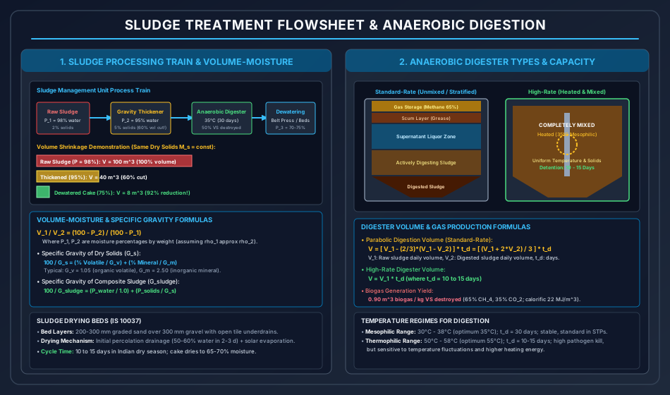
Sludge Treatment Flowsheet & Anaerobic Digestion

3.1 Sources & Types of Wastewater Sludge

  1. Primary Sludge: Settleable solids removed in the Primary Settling Tank (PST). Greyish, fibrous, highly putrescible; moisture content P=95%−97.5%P = 95\% - 97.5\% (2.5%−5%2.5\% - 5\% solids).
  2. Secondary / Waste Activated Sludge (WAS): Biological flocs wasted from secondary clarifiers. Brownish, gelatinous, microbial cell tissue; exceptionally high moisture content P=98%−99.5%P = 98\% - 99.5\% (0.5%−2%0.5\% - 2\% solids); difficult to dewater without chemical conditioning.
  3. Chemical Sludge: Precipitates formed during chemical coagulation (alum, ferric salts, lime). Dense, gelatinous; moisture content 96%−98%96\% - 98\%.

3.2 Specific Gravity of Sludge & Solids

Sludge consists of mineral matter (fixed solids, FS, Gm≈2.50G_m \approx 2.50) and organic matter (volatile solids, VS, Gv≈1.05G_v \approx 1.05).
The specific gravity of dry composite solids (GsG_s) is:

100Gs=% Volatile SolidsGv+% Mineral SolidsGm\frac{100}{G_s} = \frac{\% \text{ Volatile Solids}}{G_v} + \frac{\% \text{ Mineral Solids}}{G_m}

For typical primary sludge (70%70\% volatile, 30%30\% mineral):

100Gs=701.05+302.50=66.67+12.00=78.67  ⟹  Gs=10078.67=1.271\frac{100}{G_s} = \frac{70}{1.05} + \frac{30}{2.50} = 66.67 + 12.00 = 78.67 \implies G_s = \frac{100}{78.67} = 1.271

The specific gravity of the wet composite sludge (GsludgeG_{\text{sludge}}) with moisture percentage PP (water specific gravity =1.00= 1.00):

100Gsludge=P1.00+100−PGs\frac{100}{G_{\text{sludge}}} = \frac{P}{1.00} + \frac{100 - P}{G_s}

For P=98.0%P = 98.0\% moisture:

100Gsludge=98.01.00+2.01.271=98.0+1.573=99.573  ⟹  Gsludge=10099.573=1.0043≈1.00\frac{100}{G_{\text{sludge}}} = \frac{98.0}{1.00} + \frac{2.0}{1.271} = 98.0 + 1.573 = 99.573 \implies G_{\text{sludge}} = \frac{100}{99.573} = 1.0043 \approx 1.00

(Because moisture exceeds 95%95\%, sludge density is practically equal to water: ρsludge≈1,000 kg/m3\rho_{\text{sludge}} \approx 1,000\text{ kg/m}^3).

3.3 The Sludge Volume-Moisture Relationship

Because the absolute mass of dry solids (MsM_s) remains unchanged during physical thickening or dewatering:

Ms=V1⋅ρ1⋅(100−P1100)=V2⋅ρ2⋅(100−P2100)M_s = V_1 \cdot \rho_1 \cdot \left(\frac{100 - P_1}{100}\right) = V_2 \cdot \rho_2 \cdot \left(\frac{100 - P_2}{100}\right)

Assuming ρ1≈ρ2≈ρw\rho_1 \approx \rho_2 \approx \rho_w:

V1(100−P1)=V2(100−P2)  ⟹  V1V2=100−P2100−P1V_1 (100 - P_1) = V_2 (100 - P_2) \implies \frac{V_1}{V_2} = \frac{100 - P_2}{100 - P_1}

Where:

  • V1,V2=V_1, V_2 = sludge volumes before and after moisture reduction (m3\text{m}^3).
  • P1,P2=P_1, P_2 = moisture percentages by weight before and after processing.
  • 100−P1,100−P2=100 - P_1, 100 - P_2 = solids percentages by weight.

[!IMPORTANT] The Golden Rule of Sludge Dewatering:
A modest drop in moisture content produces an enormous contraction in sludge volume!

  • Thickening from 98%98\% to 96%96\% moisture: V2V1=100−98100−96=24=0.50  ⟹  50% volume reduction!\frac{V_2}{V_1} = \frac{100 - 98}{100 - 96} = \frac{2}{4} = 0.50 \implies \mathbf{50\% \text{ volume reduction!}}
  • Dewatering from 98%98\% to 75%75\% (cake): V3V1=100−98100−75=225=0.08  ⟹  92% volume reduction!\frac{V_3}{V_1} = \frac{100 - 98}{100 - 75} = \frac{2}{25} = 0.08 \implies \mathbf{92\% \text{ volume reduction!}}

4. Sludge Thickening & Conditioning

4.1 Sludge Thickening Processes

  1. Gravity Thickeners:
    • Circular tanks equipped with slowly rotating vertical pickets / stirrers (vtip≈0.05 m/sv_{\text{tip}} \approx 0.05\text{ m/s}).
    • The picket fence mechanism creates gentle vertical channels that release trapped water and gas bubbles, compacting primary sludge from 2%2\% to 5−8%5 - 8\% solids (98%→92−95%98\% \to 92 - 95\% moisture).
    • Solids loading rate: 30−60 kg solids/m2⋅day30 - 60\text{ kg solids/m}^2\cdot\text{day}.
  2. Dissolved Air Flotation (DAF):
    • Ideal for light biological waste activated sludge (WAS) which resists gravity settling.
    • Air is dissolved in recycled effluent under pressure (300−500 kPa300 - 500\text{ kPa}); when injected into the flotation tank, tiny micro-bubbles (30−80 μm30 - 80\,\mu\text{m}) attach to sludge flocs, floating them to the surface where mechanical skimmers harvest a 4−6%4 - 6\% solids cake.
  3. Centrifugal Thickeners: Continuous solid-bowl decanter centrifuges using centrifugal acceleration (1,000−3,000×g1,000 - 3,000 \times g).

4.2 Sludge Conditioning

To destabilize bound water and agglomerate colloidal biological particles prior to mechanical dewatering:

  • Chemical Conditioning: Addition of inorganic coagulants (FeCl3\text{FeCl}_3, lime) or high-molecular-weight cationic synthetic polymers (polyelectrolytes, 2−6 kg/tonne dry solids2 - 6\text{ kg/tonne dry solids}).
  • Elutriation (Washing): Washing digested sludge with plant effluent to wash out soluble alkaline bicarbonates and reduce coagulant chemical demand.

5. Anaerobic Sludge Digestion Engineering

Anaerobic digestion biochemically stabilizes concentrated organic solids into odorless humic matter, destroying pathogenic bacteria and generating renewable methane biogas.

5.1 Environmental Operating Regimes

  1. Mesophilic Digestion:
    • Operating temperature: 35∘C±2∘C35^\circ\text{C} \pm 2^\circ\text{C} (30∘C−38∘C30^\circ\text{C} - 38^\circ\text{C}).
    • Digestion detention time: 30−40 days30 - 40\text{ days} (standard-rate) or 15−20 days15 - 20\text{ days} (high-rate).
    • Highly robust, commercially dominant standard worldwide.
  2. Thermophilic Digestion:
    • Operating temperature: 55∘C±2∘C55^\circ\text{C} \pm 2^\circ\text{C} (50∘C−58∘C50^\circ\text{C} - 58^\circ\text{C}).
    • Digestion detention time: 10−15 days10 - 15\text{ days}.
    • Faster reaction rates and complete pathogen sterilization, but sensitive to thermal shocks and produces odors.

5.2 Reactor Configurations: Standard-Rate vs High-Rate

  • Standard-Rate Digester (Conventional / Stratified):
    • Unheated, unmixed; single cylindrical tank with floating gas holder cover.
    • Stratifies into 4 distinct physical zones:
      1. Top Scum Layer: Hard mat of grease, hair, and floating buoyant debris.
      2. Supernatant Zone: High-strength ammoniacal liquor recycled back to STP inlet.
      3. Actively Digesting Sludge Layer: Active bacterial consortia decomposing organics.
      4. Stabilized Bottom Sludge: Mineralized black sludge ready for dewatering.
    • Sludge detention time: 30−60 days30 - 60\text{ days}.
  • High-Rate Digester:
    • Heated to 35∘C35^\circ\text{C} via external spiral heat exchangers; completely mixed via internal mechanical draft-tube impellers or compressed biogas injection.
    • Completely homogeneous (no stratification, no supernatant separation).
    • Sludge detention time: 10−15 days10 - 15\text{ days}.

5.3 Digester Capacity Formulation

In a standard-rate digester, sludge volume decreases continuously from daily incoming volume V1V_1 to digested volume V2V_2. Because gas release and volume contraction follow a parabolic decay:

Vdigester=[V1−23(V1−V2)]td=[V1+2V23]tdV_{\text{digester}} = \left[ V_1 - \frac{2}{3}(V_1 - V_2) \right] t_d = \left[ \frac{V_1 + 2 V_2}{3} \right] t_d

Where:

  • V1=V_1 = daily volume of raw sludge added (m3/day\text{m}^3/\text{day}).
  • V2=V_2 = daily volume of digested sludge produced (m3/day\text{m}^3/\text{day}).
  • td=t_d = statutory digestion period in days (typically 30 days30\text{ days} at 35∘C35^\circ\text{C}).

5.4 Biogas Energy Yield

During anaerobic digestion, approximately 50%−55%50\% - 55\% of volatile solids are destroyed:

Biogas Production=0.90 m3/kg volatile solids destroyed\text{Biogas Production} = 0.90\text{ m}^3 / \text{kg volatile solids destroyed}
  • Typical Biogas Composition: 65% CH465\% \text{ CH}_4 (methane), 30−35% CO230 - 35\% \text{ CO}_2, trace H2S\text{H}_2\text{S}.
  • Net calorific value of biogas: 20−22 MJ/m320 - 22\text{ MJ/m}^3 (pure methane =35.8 MJ/m3= 35.8\text{ MJ/m}^3).

6. Sludge Dewatering & Final Disposal

  1. Open Sludge Drying Beds (IS 10037 Part 1):
    • Underdrained sand filter beds: 200−300 mm200 - 300\text{ mm} graded sand (d10=0.3−0.5 mm,Cu≤4.0d_{10} = 0.3 - 0.5\text{ mm}, C_u \le 4.0) overlying 300 mm300\text{ mm} graded gravel, laid with open-jointed vitrified clay tile drains on 1:1001:100 bed slope.
    • Dewatering Mechanisms: (i) Gravity drainage of free water (50−60%50-60\% water drained in first 2-3 days); (ii) Solar radiation evaporation.
    • Sludge applied in 200−250 mm200 - 250\text{ mm} liquid cakes; dries in 10−15 days10 - 15\text{ days} in dry weather to cracked spadeable cake (65−70%65 - 70\% moisture).
  2. Mechanical Dewatering Systems:
    • Belt Filter Press (BFP): Continuous porous belts squeezing sludge through diminishing-diameter rollers (18−25%18 - 25\% dry solids cake).
    • Centrifuges (Decanters): High G-force spin separating cake from centrate (20−30%20 - 30\% solids).
    • Plate-and-Frame Filter Press: High-pressure hydraulic chambers (7−15 bar7 - 15\text{ bar}) yielding dense cakes (35−45%35 - 45\% solids).
  3. Ultimate Disposal:
    • Agricultural land application / composting (valuable soil conditioner rich in N, P\text{N, P}; regulated for heavy metals per IS standards).
    • Co-processing in cement kilns / incineration.
    • Engineered sanitary landfilling.

7. River Stream Self-Purification & Ecological Zones

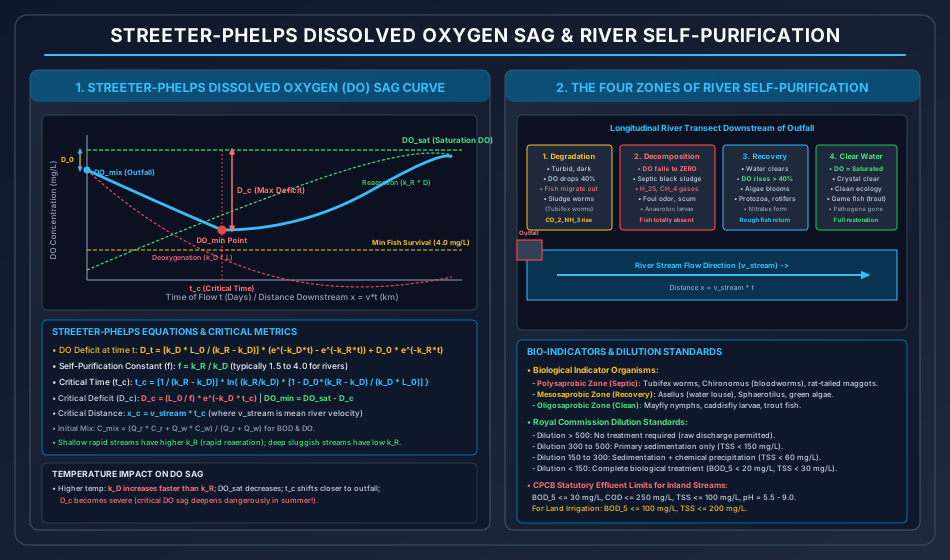
Streeter-Phelps DO Sag & River Self-Purification

7.1 Hydrodynamic Initial Mix at Outfall

When treated wastewater discharge (QwQ_w) with BOD concentration LwL_w and dissolved oxygen DOwDO_w mixes completely with upstream river flow (Qr,Lr,DOrQ_r, L_r, DO_r):

Combined Mixed Discharge Qmix=Qr+Qw\text{Combined Mixed Discharge } Q_{\text{mix}} = Q_r + Q_w Initial Mixed Ultimate BOD L0=QrLr+QwLwQr+Qw\text{Initial Mixed Ultimate BOD } L_0 = \frac{Q_r L_r + Q_w L_w}{Q_r + Q_w} Initial Mixed Dissolved Oxygen DOmix=QrDOr+QwDOwQr+Qw\text{Initial Mixed Dissolved Oxygen } DO_{\text{mix}} = \frac{Q_r DO_r + Q_w DO_w}{Q_r + Q_w} Initial Oxygen Deficit D0=DOsat−DOmix\text{Initial Oxygen Deficit } D_0 = DO_{\text{sat}} - DO_{\text{mix}}

Where DOsatDO_{\text{sat}} is saturation dissolved oxygen concentration at stream temperature (9.17 mg/L9.17\text{ mg/L} at 20∘C20^\circ\text{C}).

7.2 The Four Ecological Zones of Stream Self-Purification

Downstream from a wastewater discharge outfall, a polluted river exhibits four progressive biological and chemical zones:

Zone of Stream Dissolved Oxygen (DO) Profile Physical Water Appearance Dominant Bio-Indicator Flora & Fauna
1. Zone of Degradation Drops sharply from saturation down to ≈40%\approx 40\% saturation. Turbid, dark grey, floating solids, scum blankets. • Sludge worms (Tubifex tubifex), Chironomid bloodworms.
• Game fish flee downstream; coarse fish tolerate stress.
2. Zone of Active Decomposition Plummets to ZERO; strictly anaerobic conditions prevail. Black septic sludge bed; bubbling foul gases (H2S,CH4\text{H}_2\text{S}, \text{CH}_4); scum mats. • Fish life completely extinct.
• Anaerobic bacteria and rat-tailed maggots (Eristalis tenax).
3. Zone of Recovery Reaeration outpaces deoxygenation; DO rises steadily above 40%40\%. Water clarifies; sunlight penetrates; black sludge mineralizes. • Algae proliferate (photosynthetic oxygenation).
• Protozoa, rotifers, water louse (Asellus aquaticus); coarse fish return.
4. Zone of Clear Water DO restored to full saturation (100%100\%). Crystal clear, odorless, stable river ecology. • Clean-water invertebrates (Mayfly nymphs, Caddisfly larvae).
• Game fish (Trout, Mahseer, Carp) fully thrive.

8. The Streeter-Phelps Dissolved Oxygen Sag Formulation

In 1925, H. W. Streeter and Earle B. Phelps formulated the simultaneous competition between microbial deoxygenation (oxygen consumption by BOD) and atmospheric reaeration (oxygen replenishment across the free water surface).

8.1 The Governing Differential Equation

At any time tt of stream travel:

dDdt=Rate of Deoxygenation−Rate of Reaeration=kD⋅Lt−kR⋅D\frac{dD}{dt} = \text{Rate of Deoxygenation} - \text{Rate of Reaeration} = k_D \cdot L_t - k_R \cdot D

Where:

  • D=DOsat−DO=D = DO_{\text{sat}} - DO = dissolved oxygen deficit at time tt (mg/L\text{mg/L}).
  • Lt=L0⋅e−kD⋅t=L_t = L_0 \cdot e^{-k_D \cdot t} = remaining ultimate carbonaceous BOD at time tt (mg/L\text{mg/L}).
  • kD=k_D = deoxygenation rate constant to base ee (day−1\text{day}^{-1}, typically 0.10−0.35 day−10.10 - 0.35\text{ day}^{-1}).
  • kR=k_R = reaeration rate constant to base ee (day−1\text{day}^{-1}, typically 0.20−1.0 day−10.20 - 1.0\text{ day}^{-1}).

Substituting Lt=L0e−kDtL_t = L_0 e^{-k_D t}:

dDdt+kR⋅D=kD⋅L0⋅e−kD⋅t\frac{dD}{dt} + k_R \cdot D = k_D \cdot L_0 \cdot e^{-k_D \cdot t}

8.2 Integrated Streeter-Phelps Equation

Integrating with initial condition D=D0D = D_0 at t=0t = 0:

Dt=kD⋅L0kR−kD(e−kD⋅t−e−kR⋅t)+D0⋅e−kR⋅t(Base e)D_t = \frac{k_D \cdot L_0}{k_R - k_D} \left( e^{-k_D \cdot t} - e^{-k_R \cdot t} \right) + D_0 \cdot e^{-k_R \cdot t} \quad (\text{Base } e)

In Base 10 notation (kD=2.303KD,kR=2.303KRk_D = 2.303 K_D, k_R = 2.303 K_R):

Dt=KD⋅L0KR−KD(10−KD⋅t−10−KR⋅t)+D0⋅10−KR⋅tD_t = \frac{K_D \cdot L_0}{K_R - K_D} \left( 10^{-K_D \cdot t} - 10^{-K_R \cdot t} \right) + D_0 \cdot 10^{-K_R \cdot t}

8.3 Critical DO Sag Point: Time (tct_c) & Deficit (DcD_c)

The critical point represents the location of maximum oxygen deficit (Dmax=DcD_{\text{max}} = D_c) and minimum dissolved oxygen (DOmin=DOsat−DcDO_{\text{min}} = DO_{\text{sat}} - D_c).
At this local mathematical extremum, the deoxygenation rate exactly balances the reaeration rate:

dDdt=0  ⟺  kD⋅Lc=kR⋅Dc\frac{dD}{dt} = 0 \iff k_D \cdot L_c = k_R \cdot D_c

Defining the stream self-purification constant ff:

f=kRkD=KRKDf = \frac{k_R}{k_D} = \frac{K_R}{K_D}

1. Critical Time (tct_c):

tc=1kR−kDln⁡[kRkD(1−D0(kR−kD)kD⋅L0)]t_c = \frac{1}{k_R - k_D} \ln \left[ \frac{k_R}{k_D} \left( 1 - \frac{D_0 (k_R - k_D)}{k_D \cdot L_0} \right) \right] tc=1KD(f−1)log⁡10[f(1−(f−1)D0L0)](Base 10)t_c = \frac{1}{K_D (f - 1)} \log_{10} \left[ f \left( 1 - (f - 1) \frac{D_0}{L_0} \right) \right] \quad (\text{Base 10})

2. Critical Distance Downstream (xcx_c):

xc=vstream⋅tcx_c = v_{\text{stream}} \cdot t_c

Where vstreamv_{\text{stream}} is the mean cross-sectional velocity of the river.

3. Critical Maximum Deficit (DcD_c):

Dc=kDkRL0⋅e−kD⋅tc=L0f⋅e−kD⋅tc=L0f⋅10−KD⋅tcD_c = \frac{k_D}{k_R} L_0 \cdot e^{-k_D \cdot t_c} = \frac{L_0}{f} \cdot e^{-k_D \cdot t_c} = \frac{L_0}{f} \cdot 10^{-K_D \cdot t_c} DOmin=DOsat−DcDO_{\text{min}} = DO_{\text{sat}} - D_c

9. Step-by-Step Analytical Derivations

9.1 Derivation of Sludge Volume-Moisture Equation

Let a volume V1V_1 of wet sludge have a moisture content P1%P_1\% by weight and density ρ1\rho_1.
The percentage of dry solid matter in this sludge is S1=100−P1%S_1 = 100 - P_1\%.
The absolute mass of dry solids in this sludge batch (MsM_s) is:

Ms=V1⋅ρ1⋅(100−P1100)(1)M_s = V_1 \cdot \rho_1 \cdot \left(\frac{100 - P_1}{100}\right) \tag{1}

After thickening or dewatering to a new volume V2V_2, the moisture content is reduced to P2%P_2\% and density becomes ρ2\rho_2.
The percentage of solids is S2=100−P2%S_2 = 100 - P_2\%.
The absolute mass of dry solids in the thickened batch is:

Ms=V2⋅ρ2⋅(100−P2100)(2)M_s = V_2 \cdot \rho_2 \cdot \left(\frac{100 - P_2}{100}\right) \tag{2}

Because physical dewatering only extracts water and does not destroy dry solid particles, the dry solid mass is conserved:

V1⋅ρ1⋅(100−P1100)=V2⋅ρ2⋅(100−P2100)(3)V_1 \cdot \rho_1 \cdot \left(\frac{100 - P_1}{100}\right) = V_2 \cdot \rho_2 \cdot \left(\frac{100 - P_2}{100}\right) \tag{3}

Canceling the factor of 100100:

V1⋅ρ1⋅(100−P1)=V2⋅ρ2⋅(100−P2)(4)V_1 \cdot \rho_1 \cdot (100 - P_1) = V_2 \cdot \rho_2 \cdot (100 - P_2) \tag{4}

Since the specific gravity of municipal sludge (G≈1.002−1.03G \approx 1.002 - 1.03) is virtually identical to water (ρ1≈ρ2≈1,000 kg/m3\rho_1 \approx \rho_2 \approx 1,000\text{ kg/m}^3):

V1(100−P1)=V2(100−P2)(5)V_1 (100 - P_1) = V_2 (100 - P_2) \tag{5}

Dividing both sides:

V1V2=100−P2100−P1■(6)\frac{V_1}{V_2} = \frac{100 - P_2}{100 - P_1} \quad \blacksquare \tag{6}

9.2 Derivation of Streeter-Phelps Integrated Deficit Equation

The net rate of change of dissolved oxygen deficit DD in a flowing stream parcel is:

dDdt=kD⋅Lt−kR⋅D(1)\frac{dD}{dt} = k_D \cdot L_t - k_R \cdot D \tag{1}

Since carbonaceous BOD decays according to first-order kinetics (Lt=L0e−kDtL_t = L_0 e^{-k_D t}):

dDdt+kR⋅D=kD⋅L0⋅e−kD⋅t(2)\frac{dD}{dt} + k_R \cdot D = k_D \cdot L_0 \cdot e^{-k_D \cdot t} \tag{2}

This is a standard first-order linear ordinary differential equation of the form dDdt+P(t)D=Q(t)\frac{dD}{dt} + P(t)D = Q(t), where P(t)=kRP(t) = k_R and Q(t)=kDL0e−kDtQ(t) = k_D L_0 e^{-k_D t}.
The integrating factor I(t)I(t) is:

I(t)=e∫kRdt=ekR⋅t(3)I(t) = e^{\int k_R dt} = e^{k_R \cdot t} \tag{3}

Multiplying Eq. (2) by ekRte^{k_R t}:

ekRtdDdt+kRekRtD=kDL0e(kR−kD)t(4)e^{k_R t} \frac{dD}{dt} + k_R e^{k_R t} D = k_D L_0 e^{(k_R - k_D) t} \tag{4} ddt(D⋅ekRt)=kDL0e(kR−kD)t(5)\frac{d}{dt}\left( D \cdot e^{k_R t} \right) = k_D L_0 e^{(k_R - k_D) t} \tag{5}

Integrating both sides with respect to tt:

D⋅ekRt=∫kDL0e(kR−kD)tdt=kDL0kR−kDe(kR−kD)t+C(6)D \cdot e^{k_R t} = \int k_D L_0 e^{(k_R - k_D) t} dt = \frac{k_D L_0}{k_R - k_D} e^{(k_R - k_D) t} + C \tag{6}

Applying the initial boundary condition at the outfall (t=0,D=D0t = 0, D = D_0):

D0⋅e0=kDL0kR−kDe0+C  ⟹  C=D0−kDL0kR−kD(7)D_0 \cdot e^0 = \frac{k_D L_0}{k_R - k_D} e^0 + C \implies C = D_0 - \frac{k_D L_0}{k_R - k_D} \tag{7}

Substituting CC back into Eq. (6):

D⋅ekRt=kDL0kR−kDe(kR−kD)t+D0−kDL0kR−kD(8)D \cdot e^{k_R t} = \frac{k_D L_0}{k_R - k_D} e^{(k_R - k_D) t} + D_0 - \frac{k_D L_0}{k_R - k_D} \tag{8}

Multiplying throughout by e−kRte^{-k_R t}:

Dt=kDL0kR−kD(e−kDt−e−kRt)+D0e−kRt■(9)D_t = \frac{k_D L_0}{k_R - k_D} \left( e^{-k_D t} - e^{-k_R t} \right) + D_0 e^{-k_R t} \quad \blacksquare \tag{9}

9.3 Derivation of Critical Time (tct_c) and Critical Deficit (DcD_c)

At the critical point of the sag curve (t=tct = t_c), the oxygen deficit reaches its maximum value (D=DcD = D_c), which requires the derivative dDdt\frac{dD}{dt} to equal zero:

dDdt∣t=tc=0(1)\left. \frac{dD}{dt} \right|_{t = t_c} = 0 \tag{1}

From the original differential equation Eq. (1) of Section 9.2:

dDdt∣tc=kDLc−kRDc=0  ⟹  kDLc=kRDc(2)\left. \frac{dD}{dt} \right|_{t_c} = k_D L_c - k_R D_c = 0 \implies k_D L_c = k_R D_c \tag{2}

Substitute Lc=L0e−kDtcL_c = L_0 e^{-k_D t_c}:

Dc=kDkRL0e−kDtc(3)D_c = \frac{k_D}{k_R} L_0 e^{-k_D t_c} \tag{3}

Differentiating the integrated equation Eq. (9) directly with respect to tt:

dDdt=kDL0kR−kD(−kDe−kDt+kRe−kRt)−kRD0e−kRt=0(4)\frac{dD}{dt} = \frac{k_D L_0}{k_R - k_D}\left( -k_D e^{-k_D t} + k_R e^{-k_R t} \right) - k_R D_0 e^{-k_R t} = 0 \tag{4} kDL0kR−kD(kRe−kRtc−kDe−kDtc)=kRD0e−kRtc(5)\frac{k_D L_0}{k_R - k_D}\left( k_R e^{-k_R t_c} - k_D e^{-k_D t_c} \right) = k_R D_0 e^{-k_R t_c} \tag{5}

Dividing both sides by e−kRtce^{-k_R t_c}:

kDL0kR−kD(kR−kDe(kR−kD)tc)=kRD0(6)\frac{k_D L_0}{k_R - k_D}\left( k_R - k_D e^{(k_R - k_D) t_c} \right) = k_R D_0 \tag{6} kR−kDe(kR−kD)tc=kRD0(kR−kD)kDL0(7)k_R - k_D e^{(k_R - k_D) t_c} = \frac{k_R D_0 (k_R - k_D)}{k_D L_0} \tag{7} kDe(kR−kD)tc=kR−kRD0(kR−kD)kDL0=kR[1−D0(kR−kD)kDL0](8)k_D e^{(k_R - k_D) t_c} = k_R - \frac{k_R D_0 (k_R - k_D)}{k_D L_0} = k_R \left[ 1 - \frac{D_0 (k_R - k_D)}{k_D L_0} \right] \tag{8} e(kR−kD)tc=kRkD[1−D0(kR−kD)kDL0](9)e^{(k_R - k_D) t_c} = \frac{k_R}{k_D} \left[ 1 - \frac{D_0 (k_R - k_D)}{k_D L_0} \right] \tag{9}

Taking the natural logarithm:

(kR−kD)tc=ln⁡{kRkD[1−D0(kR−kD)kDL0]}(10)(k_R - k_D) t_c = \ln \left\{ \frac{k_R}{k_D} \left[ 1 - \frac{D_0 (k_R - k_D)}{k_D L_0} \right] \right\} \tag{10} tc=1kR−kDln⁡{kRkD[1−D0(kR−kD)kDL0]}■(11)t_c = \frac{1}{k_R - k_D} \ln \left\{ \frac{k_R}{k_D} \left[ 1 - \frac{D_0 (k_R - k_D)}{k_D L_0} \right] \right\} \quad \blacksquare \tag{11}

10. Solved Numerical Example 1: Sludge Thickening, Dewatering & S.G.

Problem Statement

A municipal wastewater treatment plant generates Mraw=12,000.0 kg/dayM_{\text{raw}} = 12,000.0\text{ kg/day} of raw primary sludge with a moisture content of P1=98.0%P_1 = 98.0\%.
Laboratory analysis shows that the dry solids consist of 70.0%70.0\% volatile organic matter (specific gravity Gv=1.05G_v = 1.05) and 30.0%30.0\% fixed mineral matter (specific gravity Gm=2.50G_m = 2.50).
The raw sludge is thickened in a gravity thickener to P2=95.0%P_2 = 95.0\% moisture, and subsequently dewatered on a belt filter press to produce a spadeable cake of P3=75.0%P_3 = 75.0\% moisture.

Calculate:

  1. The specific gravity of the dry solids (GsG_s) and the specific gravity of the raw sludge (GsludgeG_{\text{sludge}}).
  2. The initial daily volume of raw sludge (V1V_1), the daily volume of thickened sludge (V2V_2), and the percentage volume reduction achieved in the thickener.
  3. The final daily volume of dewatered cake (V3V_3) and the overall total percentage volume reduction from raw sludge to final dewatered cake.

Complete Analytical Solution

1. Specific Gravity of Dry Solids (GsG_s) & Sludge (GsludgeG_{\text{sludge}})

100Gs=% VolatileGv+% MineralGm=70.01.05+30.02.50=66.6667+12.0000=78.6667\frac{100}{G_s} = \frac{\% \text{ Volatile}}{G_v} + \frac{\% \text{ Mineral}}{G_m} = \frac{70.0}{1.05} + \frac{30.0}{2.50} = 66.6667 + 12.0000 = 78.6667 Gs=10078.6667=1.27119≈1.2712G_s = \frac{100}{78.6667} = 1.27119 \approx 1.2712

Specific gravity of wet raw sludge (98.0%98.0\% water):

100Gsludge=P11.00+100−P1Gs=98.01.00+2.01.27119=98.0+1.5733=99.5733\frac{100}{G_{\text{sludge}}} = \frac{P_1}{1.00} + \frac{100 - P_1}{G_s} = \frac{98.0}{1.00} + \frac{2.0}{1.27119} = 98.0 + 1.5733 = 99.5733 Gsludge=10099.5733=1.00428≈1.0043G_{\text{sludge}} = \frac{100}{99.5733} = 1.00428 \approx 1.0043

2. Raw Volume (V1V_1), Thickened Volume (V2V_2) & Volume Reduction

Daily mass of dry solids (MsM_s):

Ms=Mraw×(1−0.98)=12,000.0×0.02=240.0 kg solids/dayM_s = M_{\text{raw}} \times (1 - 0.98) = 12,000.0 \times 0.02 = 240.0\text{ kg solids/day}

Volume of raw sludge (V1V_1):

V1=Mrawρsludge=12,000.0 kg/day1.00428×1,000 kg/m3=11.9488 m3/day≈11.95 m3/dayV_1 = \frac{M_{\text{raw}}}{\rho_{\text{sludge}}} = \frac{12,000.0\text{ kg/day}}{1.00428 \times 1,000\text{ kg/m}^3} = 11.9488\text{ m}^3/\text{day} \approx 11.95\text{ m}^3/\text{day}

Applying the volume-moisture relationship for gravity thickening to P2=95.0%P_2 = 95.0\%:

V2=V1⋅(100−P1100−P2)=11.9488×(100−98.0100−95.0)=11.9488×2.05.0=4.7795 m3/day≈4.78 m3/dayV_2 = V_1 \cdot \left(\frac{100 - P_1}{100 - P_2}\right) = 11.9488 \times \left(\frac{100 - 98.0}{100 - 95.0}\right) = 11.9488 \times \frac{2.0}{5.0} = 4.7795\text{ m}^3/\text{day} \approx 4.78\text{ m}^3/\text{day}

Thickener volume reduction:

Reductionthick=V1−V2V1×100=11.9488−4.779511.9488×100=60.00%\text{Reduction}_{\text{thick}} = \frac{V_1 - V_2}{V_1} \times 100 = \frac{11.9488 - 4.7795}{11.9488} \times 100 = 60.00\%

3. Dewatered Cake Volume (V3V_3) & Overall Reduction

Dewatering to P3=75.0%P_3 = 75.0\% moisture:

V3=V1⋅(100−P1100−P3)=11.9488×(100−98.0100−75.0)=11.9488×2.025.0=0.9559 m3/day≈0.956 m3/dayV_3 = V_1 \cdot \left(\frac{100 - P_1}{100 - P_3}\right) = 11.9488 \times \left(\frac{100 - 98.0}{100 - 75.0}\right) = 11.9488 \times \frac{2.0}{25.0} = 0.9559\text{ m}^3/\text{day} \approx 0.956\text{ m}^3/\text{day}

Overall volume reduction from raw liquid sludge to spadeable cake:

Reductiontotal=V1−V3V1×100=11.9488−0.955911.9488×100=10.992911.9488×100=92.00%\text{Reduction}_{\text{total}} = \frac{V_1 - V_3}{V_1} \times 100 = \frac{11.9488 - 0.9559}{11.9488} \times 100 = \frac{10.9929}{11.9488} \times 100 = 92.00\%

11. Solved Numerical Example 2: Anaerobic Digester Sizing & Biogas Generation

Problem Statement

A municipal wastewater treatment plant produces V1=40.0 m3/dayV_1 = 40.0\text{ m}^3/\text{day} of raw primary sludge having a moisture content of 96.0%96.0\% (4.0%4.0\% dry solids).
The dry solids contain 70.0%70.0\% volatile solids. The sludge is stabilized in a standard-rate mesophilic anaerobic digester operated at 35∘C35^\circ\text{C} with a digestion retention period of td=30.0 dayst_d = 30.0\text{ days}.
Anaerobic digestion achieves a 50.0%50.0\% reduction in volatile solids. The digested sludge drawn from the bottom hopper has a moisture content of 92.0%92.0\% (8.0%8.0\% solids).

Calculate:

  1. The mass of dry solids and volatile solids entering the digester daily.
  2. The mass of digested dry solids produced daily and the daily volume of digested sludge (V2V_2).
  3. The design volume of the anaerobic digester (VV) assuming parabolic volume contraction.
  4. The daily total volume of biogas and methane gas generated, given a gas yield of 0.90 m3 biogas / kg volatile solids destroyed0.90\text{ m}^3 \text{ biogas / kg volatile solids destroyed} with 65.0%65.0\% methane content.

Complete Analytical Solution

1. Daily Raw Sludge Solids Breakdown

Raw sludge flow V1=40.0 m3/dayV_1 = 40.0\text{ m}^3/\text{day}, moisture P1=96.0%  ⟹  4.0%P_1 = 96.0\% \implies 4.0\% solids.
Assuming ρ≈1,000 kg/m3\rho \approx 1,000\text{ kg/m}^3:

Total Raw Solids Ms=40.0 m3/day×1,000 kg/m3×0.04=1,600.0 kg solids/day\text{Total Raw Solids } M_s = 40.0\text{ m}^3/\text{day} \times 1,000\text{ kg/m}^3 \times 0.04 = 1,600.0\text{ kg solids/day} Volatile Solids (VS)=0.70×1,600.0=1,120.0 kg VS/day\text{Volatile Solids (VS)} = 0.70 \times 1,600.0 = 1,120.0\text{ kg VS/day} Fixed Mineral Solids (FS)=0.30×1,600.0=480.0 kg FS/day\text{Fixed Mineral Solids (FS)} = 0.30 \times 1,600.0 = 480.0\text{ kg FS/day}

2. Digested Sludge Solids & Volume (V2V_2)

Digestion destroys 50.0%50.0\% of volatile solids:

VS Destroyed=0.50×1,120.0=560.0 kg VS/day\text{VS Destroyed} = 0.50 \times 1,120.0 = 560.0\text{ kg VS/day} VS Remaining=1,120.0−560.0=560.0 kg VS/day\text{VS Remaining} = 1,120.0 - 560.0 = 560.0\text{ kg VS/day}

Fixed mineral solids pass through unaffected:

FS Remaining=480.0 kg FS/day\text{FS Remaining} = 480.0\text{ kg FS/day} Total Digested Dry Solids Ms,dig=560.0+480.0=1,040.0 kg solids/day\text{Total Digested Dry Solids } M_{s,\text{dig}} = 560.0 + 480.0 = 1,040.0\text{ kg solids/day}

Digested sludge moisture P2=92.0%  ⟹  8.0%P_2 = 92.0\% \implies 8.0\% solids:

V2=Ms,digρ×(1−P2/100)=1,040.0 kg/day1,000 kg/m3×0.08=13.00 m3/dayV_2 = \frac{M_{s,\text{dig}}}{\rho \times (1 - P_2/100)} = \frac{1,040.0\text{ kg/day}}{1,000\text{ kg/m}^3 \times 0.08} = 13.00\text{ m}^3/\text{day}

3. Anaerobic Digester Capacity (VV)

Applying the parabolic volume reduction equation for standard-rate digesters (td=30 dayst_d = 30\text{ days}):

Vavg=V1−23(V1−V2)=40.0−23(40.0−13.0)=40.0−23(27.0)=40.0−18.0=22.00 m3/dayV_{\text{avg}} = V_1 - \frac{2}{3}(V_1 - V_2) = 40.0 - \frac{2}{3}(40.0 - 13.0) = 40.0 - \frac{2}{3}(27.0) = 40.0 - 18.0 = 22.00\text{ m}^3/\text{day} V=Vavg⋅td=22.00 m3/day×30.0 days=660.00 m3≈660.0 m3V = V_{\text{avg}} \cdot t_d = 22.00\text{ m}^3/\text{day} \times 30.0\text{ days} = 660.00\text{ m}^3 \approx 660.0\text{ m}^3

4. Biogas & Methane Production

Daily VS Destroyed=560.0 kg VS/day\text{Daily VS Destroyed} = 560.0\text{ kg VS/day} Total Biogas=560.0 kg VS/day×0.90 m3/kg=504.0 m3/day\text{Total Biogas} = 560.0\text{ kg VS/day} \times 0.90\text{ m}^3/\text{kg} = 504.0\text{ m}^3/\text{day} Methane Gas (CH4)=0.65×504.0=327.60 m3/day≈327.6 m3/day\text{Methane Gas } (\text{CH}_4) = 0.65 \times 504.0 = 327.60\text{ m}^3/\text{day} \approx 327.6\text{ m}^3/\text{day}

12. Solved Numerical Example 3: Streeter-Phelps River DO Sag Analysis

Problem Statement

A treated municipal wastewater effluent is discharged into a freshwater river stream. The operating data are:

  • Effluent: Discharge Qw=1.50 m3/sQ_w = 1.50\text{ m}^3/\text{s}, 5-day BOD BOD5,w=40.0 mg/L\text{BOD}_{5,w} = 40.0\text{ mg/L} (kD=0.230 day−1k_D = 0.230\text{ day}^{-1}), Dissolved Oxygen DOw=2.00 mg/LDO_w = 2.00\text{ mg/L}.
  • River: Flow Qr=8.50 m3/sQ_r = 8.50\text{ m}^3/\text{s}, Ultimate BOD Lr=3.00 mg/LL_r = 3.00\text{ mg/L}, Dissolved Oxygen DOr=8.50 mg/LDO_r = 8.50\text{ mg/L}, Mean flow velocity v=0.250 m/sv = 0.250\text{ m/s}.
  • Saturated DO at river temperature (20∘C20^\circ\text{C}): DOsat=9.17 mg/LDO_{\text{sat}} = 9.17\text{ mg/L}.
  • Kinetic rates (to Base ee): Deoxygenation kD=0.230 day−1k_D = 0.230\text{ day}^{-1}, Reaeration kR=0.460 day−1k_R = 0.460\text{ day}^{-1} (f=kR/kD=2.00f = k_R / k_D = 2.00).

Calculate:

  1. The initial combined discharge (QmixQ_{\text{mix}}), initial ultimate BOD (L0L_0), initial mixed DO, and initial DO deficit (D0D_0) at the outfall.
  2. The critical time of travel (tct_c in days and hours) and the critical distance downstream (xcx_c in kilometers).
  3. The critical maximum DO deficit (DcD_c) and the minimum stream dissolved oxygen (DOminDO_{\text{min}}).
  4. Evaluate whether the minimum DO satisfies the statutory threshold for cold-water fish survival (DO≥4.0 mg/LDO \ge 4.0\text{ mg/L}).

Complete Analytical Solution

1. Outfall Mixing Conditions (t=0t = 0)

Ultimate BOD of wastewater (LwL_w):

Lw=BOD5,w1−e−kD×5=40.01−e−0.230×5=40.01−e−1.150=40.00.68336=58.534 mg/LL_w = \frac{\text{BOD}_{5,w}}{1 - e^{-k_D \times 5}} = \frac{40.0}{1 - e^{-0.230 \times 5}} = \frac{40.0}{1 - e^{-1.150}} = \frac{40.0}{0.68336} = 58.534\text{ mg/L}

Total mixed stream discharge:

Qmix=Qr+Qw=8.50+1.50=10.00 m3/sQ_{\text{mix}} = Q_r + Q_w = 8.50 + 1.50 = 10.00\text{ m}^3/\text{s}

Initial mixed ultimate BOD (L0L_0):

L0=QrLr+QwLwQmix=(8.50×3.00)+(1.50×58.534)10.00=25.50+87.80110.00=11.330 mg/L≈11.33 mg/LL_0 = \frac{Q_r L_r + Q_w L_w}{Q_{\text{mix}}} = \frac{(8.50 \times 3.00) + (1.50 \times 58.534)}{10.00} = \frac{25.50 + 87.801}{10.00} = 11.330\text{ mg/L} \approx 11.33\text{ mg/L}

Initial mixed dissolved oxygen (DOmixDO_{\text{mix}}):

DOmix=QrDOr+QwDOwQmix=(8.50×8.50)+(1.50×2.00)10.00=72.25+3.0010.00=7.525 mg/L≈7.53 mg/LDO_{\text{mix}} = \frac{Q_r DO_r + Q_w DO_w}{Q_{\text{mix}}} = \frac{(8.50 \times 8.50) + (1.50 \times 2.00)}{10.00} = \frac{72.25 + 3.00}{10.00} = 7.525\text{ mg/L} \approx 7.53\text{ mg/L}

Initial DO deficit (D0D_0):

D0=DOsat−DOmix=9.17−7.525=1.645 mg/L≈1.64 mg/LD_0 = DO_{\text{sat}} - DO_{\text{mix}} = 9.17 - 7.525 = 1.645\text{ mg/L} \approx 1.64\text{ mg/L}

2. Critical Time (tct_c) & Critical Distance (xcx_c)

kD=0.230 day−1,kR=0.460 day−1  ⟹  kR−kD=0.460−0.230=0.230 day−1k_D = 0.230\text{ day}^{-1}, \quad k_R = 0.460\text{ day}^{-1} \implies k_R - k_D = 0.460 - 0.230 = 0.230\text{ day}^{-1} f=kRkD=0.4600.230=2.00f = \frac{k_R}{k_D} = \frac{0.460}{0.230} = 2.00

Using the Streeter-Phelps critical time equation:

tc=1kR−kDln⁡[kRkD(1−D0(kR−kD)kD⋅L0)]t_c = \frac{1}{k_R - k_D} \ln \left[ \frac{k_R}{k_D} \left( 1 - \frac{D_0 (k_R - k_D)}{k_D \cdot L_0} \right) \right] D0(kR−kD)kD⋅L0=1.645×0.2300.230×11.330=1.64511.330=0.14519\frac{D_0 (k_R - k_D)}{k_D \cdot L_0} = \frac{1.645 \times 0.230}{0.230 \times 11.330} = \frac{1.645}{11.330} = 0.14519 1−0.14519=0.854811 - 0.14519 = 0.85481 kRkD×0.85481=2.00×0.85481=1.70962\frac{k_R}{k_D} \times 0.85481 = 2.00 \times 0.85481 = 1.70962 ln⁡(1.70962)=0.53627\ln(1.70962) = 0.53627 tc=0.536270.230=2.3316 days≈2.332 days(55.96 hours)t_c = \frac{0.53627}{0.230} = 2.3316\text{ days} \approx 2.332\text{ days} \quad (55.96\text{ hours})

Critical distance downstream (xcx_c):

xc=v⋅tc=0.250 m/s×(2.3316×86,400 s)=0.250×201,450.2=50,362.6 m≈50.36 kmx_c = v \cdot t_c = 0.250\text{ m/s} \times (2.3316 \times 86,400\text{ s}) = 0.250 \times 201,450.2 = 50,362.6\text{ m} \approx 50.36\text{ km}

3. Critical Deficit (DcD_c) & Minimum Stream DO

Dc=L0f⋅e−kD⋅tc=11.3302.00⋅e−0.230×2.3316D_c = \frac{L_0}{f} \cdot e^{-k_D \cdot t_c} = \frac{11.330}{2.00} \cdot e^{-0.230 \times 2.3316} kD⋅tc=0.230×2.3316=0.53627k_D \cdot t_c = 0.230 \times 2.3316 = 0.53627 e−0.53627=0.58493e^{-0.53627} = 0.58493 Dc=5.665×0.58493=3.3136 mg/L≈3.31 mg/LD_c = 5.665 \times 0.58493 = 3.3136\text{ mg/L} \approx 3.31\text{ mg/L}

Minimum stream DO:

DOmin=DOsat−Dc=9.17−3.3136=5.8564 mg/L≈5.86 mg/LDO_{\text{min}} = DO_{\text{sat}} - D_c = 9.17 - 3.3136 = 5.8564\text{ mg/L} \approx 5.86\text{ mg/L}

4. Environmental Life Compliance

DOmin=5.86 mg/L≥4.0 mg/LDO_{\text{min}} = 5.86\text{ mg/L} \ge 4.0\text{ mg/L}

Because the minimum dissolved oxygen along the entire river reach exceeds 4.0 mg/L4.0\text{ mg/L}, aquatic ecology and fish life are safely sustained without experiencing hypoxic distress.


13. Common Misconceptions & Exam Traps

[!WARNING] Trap 1: The Volume-Moisture Percentage Fallacy
Candidates frequently believe that reducing sludge moisture from 98%98\% to 96%96\% reduces the sludge volume by only 2%2\%.
In reality, volume depends on the solids concentration, not water concentration! Solids double from 2%2\% to 4%4\%, so volume is halved (50%50\% cut). Always write V1(100−P1)=V2(100−P2)V_1(100 - P_1) = V_2(100 - P_2).

[!WARNING] Trap 2: Base ee vs Base 10 in Streeter-Phelps
Ensure the deoxygenation and reaeration constants are matched:

  • If using e−kDte^{-k_D t}, use kDk_D and kRk_R (Napierian rates).
  • If using 10−KDt10^{-K_D t}, use KDK_D and KRK_R (Common rates, where k=2.303Kk = 2.303 K).
    Mixing kDk_D with 10−kt10^{-k t} produces catastrophic mathematical errors in tct_c and DcD_c.

[!CAUTION] Trap 3: Omitting Initial Deficit (D0D_0) at Outfall
Students often assume D0=0D_0 = 0 at the mixing point. Unless the river upstream and effluent are both 100%100\% saturated with oxygen, an initial deficit always exists:

D0=DOsat−DOmixD_0 = DO_{\text{sat}} - DO_{\text{mix}}

Neglecting D0D_0 shifts the critical time tct_c too far downstream and underestimates the critical deficit DcD_c.

[!IMPORTANT] Trap 4: Parabolic Sludge Digester Sizing Factor (2/32/3)
In standard-rate anaerobic digesters, candidate errors frequently occur when computing the average daily sludge volume:

Vavg=V1−23(V1−V2)=V1+2V23V_{\text{avg}} = V_1 - \frac{2}{3}(V_1 - V_2) = \frac{V_1 + 2 V_2}{3}

Do NOT use linear averaging V1+V22\frac{V_1 + V_2}{2}! Sludge contracts rapidly at the beginning of digestion, making the average volume significantly smaller than a linear midpoint.

[!NOTE] Trap 5: CPCB Effluent Limits for Stream Discharge
Statutory limits per CPCB for discharge into inland surface waters:

  • BOD5≤30 mg/L\text{BOD}_5 \le 30\text{ mg/L}
  • COD≤250 mg/L\text{COD} \le 250\text{ mg/L}
  • TSS≤100 mg/L\text{TSS} \le 100\text{ mg/L} For land disposal (irrigation), BOD5≤100 mg/L\text{BOD}_5 \le 100\text{ mg/L} is permitted.

14. Quick Revision Summary & Formula Sheet

14.1 Governing Mathematical Formulas

  1. Sludge Volume-Moisture Conservation: V1(100−P1)=V2(100−P2)  ⟹  V1V2=100−P2100−P1V_1 (100 - P_1) = V_2 (100 - P_2) \implies \frac{V_1}{V_2} = \frac{100 - P_2}{100 - P_1}
  2. Specific Gravity of Dry Solids (GsG_s): 100Gs=% VolatileGv+% MineralGm\frac{100}{G_s} = \frac{\% \text{ Volatile}}{G_v} + \frac{\% \text{ Mineral}}{G_m}
  3. Standard-Rate Digester Capacity: Vdigester=[V1+2V23]tdV_{\text{digester}} = \left[ \frac{V_1 + 2 V_2}{3} \right] t_d
  4. Biogas Generation: Biogas=0.90 m3/kg volatile solids destroyed(65% CH4)\text{Biogas} = 0.90\text{ m}^3 / \text{kg volatile solids destroyed} \quad (65\% \text{ CH}_4)
  5. Initial Hydrodynamic Mixing: L0=QrLr+QwLwQr+Qw,DOmix=QrDOr+QwDOwQr+Qw,D0=DOsat−DOmixL_0 = \frac{Q_r L_r + Q_w L_w}{Q_r + Q_w}, \quad DO_{\text{mix}} = \frac{Q_r DO_r + Q_w DO_w}{Q_r + Q_w}, \quad D_0 = DO_{\text{sat}} - DO_{\text{mix}}
  6. Streeter-Phelps DO Deficit Equation: Dt=kDL0kR−kD(e−kDt−e−kRt)+D0e−kRtD_t = \frac{k_D L_0}{k_R - k_D} \left( e^{-k_D t} - e^{-k_R t} \right) + D_0 e^{-k_R t}
  7. Critical Time (tct_c): tc=1kR−kDln⁡[kRkD(1−D0(kR−kD)kDL0)]t_c = \frac{1}{k_R - k_D} \ln \left[ \frac{k_R}{k_D} \left( 1 - \frac{D_0 (k_R - k_D)}{k_D L_0} \right) \right]
  8. Critical Deficit (DcD_c): Dc=L0fe−kDtc,f=kRkD,DOmin=DOsat−DcD_c = \frac{L_0}{f} e^{-k_D t_c}, \quad f = \frac{k_R}{k_D}, \quad DO_{\text{min}} = DO_{\text{sat}} - D_c

14.2 High-Yield Exam Memorization Matrix

Feature / Standard Statutory Value / Engineering Rule
Primary Sludge Moisture 95%−97.5%95\% - 97.5\% (thickens to 92%−95%92\% - 95\%).
Waste Activated Sludge (WAS) Moisture 98%−99.5%98\% - 99.5\% (thickens via DAF to 94%−96%94\% - 96\%).
Mesophilic Digestion 35∘C35^\circ\text{C} (optimum); td=30 dayst_d = 30\text{ days} (standard-rate) or 15 days15\text{ days} (high-rate).
Thermophilic Digestion 55∘C55^\circ\text{C}; td=10−15 dayst_d = 10 - 15\text{ days} (fast, heat-intensive).
Methane Content in Biogas 65% CH4,35% CO265\% \text{ CH}_4, 35\% \text{ CO}_2 (calorific value ≈22 MJ/m3\approx 22\text{ MJ/m}^3).
Fish Survival DO Threshold Minimum 4.0 mg/L4.0\text{ mg/L} dissolved oxygen.
River Zone with Zero DO Zone of Active Decomposition (black septic sludge, Tubifex worms absent).
Self-Purification Ratio (ff) f=kR/kDf = k_R / k_D (typically 1.5−4.01.5 - 4.0; higher in fast shallow streams).
CPCB Inland Effluent Discharge Limits BOD5≤30 mg/L,COD≤250 mg/L,TSS≤100 mg/L\text{BOD}_5 \le 30\text{ mg/L}, \text{COD} \le 250\text{ mg/L}, \text{TSS} \le 100\text{ mg/L}.