Water Conveyance, Distribution Networks & Service Reservoirs
In this chapter (1 topics)
On this page
- 1. Topic Title & Authoritative References
- 2. Prerequisites & Learning Objectives
- Prerequisites
- Learning Objectives
- 3. Water Transmission & Pipe Hydraulics
- 3.1 Resistance Formulations for Pipe Flow
- 3.2 Equivalent Pipe Systems
- 4. Distribution Network Configurations & Layout Analysis
- 5. Hardy Cross Loop & Nodal Flow Balancing Method
- 5.1 Fundamental Governing Principles
- 5.2 Derivation of Loop Head Correction (Δ Q)
- 6. Service Reservoirs: ESR, GSR & Mass Curve Capacity Analysis
- 6.1 Functional Purpose & Reservoir Classification
- 6.2 Minimum Residual Pressure Heads (CPHEEO Standards)
- 6.3 Components of Total Storage Capacity
- 6.4 Mass Curve (Ripple) Method Formulation
- 7. Pipeline Profile Hydraulics, Negative Head & Appurtenances
- 7.1 Hydraulic Gradient Line (HGL) vs Ground Profile
- 7.2 Functional Siting of Pipeline Appurtenances
- 8. Water Hammer Dynamics & Surge Mitigation
- 8.1 Physical Mechanism of Water Hammer
- 8.2 Acoustic Wave Velocity (c)
- 8.3 Classification of Valve Closure: Rapid vs Slow
- 8.4 Surge Mitigation Engineering Devices
- 9. Step-by-Step Analytical Derivations
- 9.1 Derivation of Hardy Cross Head Loss Correction Equation (Δ Q)
- 9.2 Derivation of Dupuit's Equivalent Pipe Formula for Pipes in Series
- 9.3 Derivation of Joukowsky Water Hammer Equation from Momentum Conservation
- 10. Solved Numerical Example 1: Equivalent Pipe System in Series
- Problem Statement
- Complete Analytical Solution
- 11. Solved Numerical Example 2: Hardy Cross Loop Network Flow Distribution
- Problem Statement
- Complete Analytical Solution
- 12. Solved Numerical Example 3: Service Reservoir Capacity by Mass Curve Method
- Problem Statement
- Complete Analytical Solution
- 13. Common Misconceptions & Exam Traps
- 14. Quick Revision Summary & Formula Sheet
- 14.1 Governing Mathematical Formulas
- 14.2 High-Yield Exam Memorization Matrix
1. Topic Title & Authoritative References
Title: Principles, Hydraulic Transmission, Network Layouts, Hardy Cross Loop Analysis, Service Reservoirs (Mass Curve Balancing Storage), Pipeline Profile Hydraulics, Appurtenances Siting, and Water Hammer Surge Dynamics.
Primary Standards & Authoritative Specifications:
- CPHEEO Manual (1999 / 2024 draft): Manual on Water Supply and Treatment, Central Public Health and Environmental Engineering Organisation, Ministry of Housing and Urban Affairs, Government of India.
- IS 779:1994: Water Meters (Domestic Type) — Specification.
- IS 14846:2000: Sluice Valves for Water Works Purposes — Specification.
- IS 12288:1987: Code of Practice for Use and Laying of Ductile Iron Pipes.
- IS 5330:1984: Criteria for Design of Anchor Blocks for Pumping Mains.
- AWWA Manual M31: Distribution Network Analysis for Water Utilities, American Water Works Association.
- AWWA Manual M51: Air-Release, Air/Vacuum, and Combination Air Valves.
- Walski, T. M., et al. (2003): Advanced Water Distribution Modeling and Management, Haestad Methods Press.
2. Prerequisites & Learning Objectives
Prerequisites
- Fluid mechanics: Continuity equation (), energy conservation (Bernoulli's theorem, HGL and TEL), Darcy-Weisbach and Hazen-Williams pipe resistance relationships.
- Vector calculus & numerical methods: Taylor series first-order truncation, Newton-Raphson method for non-linear algebraic system convergence.
- Unsteady flow dynamics: Acoustic wave mechanics, momentum flux conservation across pressure discontinuities (Joukowsky surge theory).
Learning Objectives
- Formulate pipe head loss relations (Darcy-Weisbach vs Hazen-Williams) and construct equivalent pipe configurations using Dupuit's formula for series and parallel pipes.
- Evaluate the four major municipal distribution network configurations (Dead-End, Gridiron, Ring, Radial) regarding hydraulic redundancy, cost, water quality stagnation, and fire-fighting reliability.
- Apply the Hardy Cross loop correction method (), rigorously tracking clockwise/counter-clockwise sign conventions and common branch corrections.
- Size balancing storage capacity of elevated service reservoirs (ESR) and ground service reservoirs (GSR) using the graphical and tabular Mass Curve (Ripple) method for 24-hour and intermittent pumping regimes.
- Evaluate hydraulic pipeline profiles relative to the Hydraulic Gradient Line (HGL), diagnose negative head siphon zones (cavitation / vapor pressure threshold at water), and specify appropriate appurtenances (air relief, scour/blow-off, check, sluice valves).
- Differentiate rapid from slow valve closure based on acoustic critical closure time () and quantify water hammer shock waves using Joukowsky's equation () alongside surge tank sizing principles.
3. Water Transmission & Pipe Hydraulics

3.1 Resistance Formulations for Pipe Flow
Water conveyance from source to treatment facilities and distribution to consumers relies on closed conduit flow under positive pressure. Head loss due to boundary friction () is quantified by two primary formulations:
1. Darcy-Weisbach Equation (Fundamental & Dimensionally Homogeneous)
Where:
- frictional head loss ()
- Darcy-Weisbach friction factor (dimensionless; note that , where is Fanning friction factor)
- pipe length ()
- internal diameter ()
- mean flow velocity ()
- volumetric discharge ()
- acceleration due to gravity ()
In general flow resistance notation:
For Darcy-Weisbach, and resistance coefficient .
2. Hazen-Williams Formula (Empirical Water Works Standard)
Used worldwide for municipal water distribution under turbulent flow of water at ordinary temperatures ():
Solving for head loss gradient :
Where:
- Hazen-Williams roughness coefficient (higher values represent smoother pipes; new DI/ductile iron , PVC/HDPE , new cast iron , 20-year aged unlined CI ).
- hydraulic radius ( for circular pipes running full).
- Flow exponent (conventionally taken as in hand calculations).
- Hydraulic resistance coefficient .
3.2 Equivalent Pipe Systems
An equivalent pipe is an imaginary uniform conduit that replaces a compound system of pipes while conveying the identical total discharge with an identical total head loss.
Pipes in Series (Compound Line)
When a pipeline consists of pipes of varying lengths and diameters connected end-to-end:
Substituting Darcy-Weisbach ():
If Hazen-Williams is applied:
Pipes in Parallel
When two nodes are linked by alternate pipe branches:
Using :
For Darcy-Weisbach ():
4. Distribution Network Configurations & Layout Analysis
Municipal water distribution networks must provide reliable, pressurized potable water to all service connections under fluctuating hourly demand and fire-fighting drafts.
| Network System | Structural Layout & Flow Pattern | Advantages & Suitability | Disadvantages & Operational Limitations | Typical Application |
|---|---|---|---|---|
| Dead-End / Tree System | Single trunk main branching into sub-mains, branch pipes, and terminating in dead ends. Single flow path. | • Lowest initial capital cost. • Straightforward hydraulic design. • Fewer sluice valves required. |
• Water stagnation at dead ends leads to chlorine decay, odor, and sediment accumulation. • Pipe bursts isolate entire downstream population. • Inadequate fire draft capacity. |
Old, haphazardly grown towns; unplanned suburban extensions. |
| Gridiron / Reticulation System | Mains, sub-mains, and branches interconnected in orthogonal loops. Water reaches any point from multiple directions. | • No dead ends; eliminates water stagnation. • High fire-flow capacity via multi-path feed. • Minimal consumer disruption during pipe repairs. |
• Higher piping length and capital cost. • Large number of sluice valves and cross-junctions. • Complex hydraulic calculation (requires iterative loop analysis). |
Well-planned cities with rectangular street grids (Chandigarh, Gandhinagar). |
| Ring / Circular System | Supply main encircles the perimeter of the district, feeding cross-branches inwards toward the center. | • High pressure maintained along periphery. • Excellent security of supply for central commercial cores. • Dual-direction feed to all internal sectors. |
• Higher circumferential main diameter and pipe length. • Requires perimeter easement/rights of way. |
Towns and sectors with radial road networks or defined commercial city centers. |
| Radial System | City divided into discrete zones; centrally placed service reservoir (ESR) in each zone pumps/distributes radially outwards. | • High and uniform terminal pressure heads. • Rapid calculation of zonal pipe sizing. • Excellent pressure zone isolation (zonal metering). |
• Requires multiple elevated service reservoirs. • Highest overall capital expenditure. |
Modern planned metropolitan layouts; high-density multi-story zoned developments. |
5. Hardy Cross Loop & Nodal Flow Balancing Method
The Hardy Cross method (1936) is an iterative numerical technique based on the Newton-Raphson approximation to solve head loss and discharge distributions in indeterminate pipe networks.
5.1 Fundamental Governing Principles
- Law of Conservation of Mass (Continuity at Nodes): At every junction node , algebraic sum of all inflows and outflows must equal zero:
- Law of Conservation of Energy (Head Balance in Closed Loops): Around any closed loop , the algebraic sum of frictional and minor head losses must equal zero:
5.2 Derivation of Loop Head Correction ()
Let an initial trial discharge be assigned to each pipe such that continuity () is satisfied at every node. If this trial flow deviates from the true converged discharge by correction :
Assuming the correction is uniform for all pipes within loop to preserve nodal continuity, the loop energy equation becomes:
Expanding via Taylor series expansion and truncating higher-order terms ():
Substituting into the loop energy balance:
Solving explicitly for the loop flow correction :
Where:
- for Darcy-Weisbach ().
- (or ) for Hazen-Williams ().
- Sign Convention: Flows in clockwise direction around the loop produce positive head losses (); counter-clockwise flows produce negative head losses ().
- If computes to a negative value, the correction is applied counter-clockwise; if positive, it is applied clockwise.
- Common Pipe Correction: For a pipe shared between Loop A and Loop B, both loop corrections apply:
6. Service Reservoirs: ESR, GSR & Mass Curve Capacity Analysis
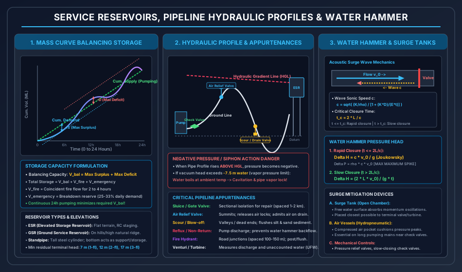
6.1 Functional Purpose & Reservoir Classification
Service reservoirs provide equalizing capacity between constant-rate treatment/pumping and fluctuating community consumer demand, while maintaining statutory residual pressure heads.
- Ground Service Reservoirs (GSR): Constructed at grade or partially submerged on high natural hills, ridges, or elevated ground. Most economical storage per cubic meter.
- Elevated Storage Reservoirs (ESR / Overhead Tanks): Built on reinforced concrete or structural steel staging ( height) over flat topography.
- Standpipes: Tall cylindrical steel or prestressed concrete tanks resting on the ground where the upper volume provides pressurized balancing storage and lower volume serves as reserve.
6.2 Minimum Residual Pressure Heads (CPHEEO Standards)
To deliver water into domestic upper-floor fixtures without booster pumps:
- Single-storey buildings: ( or )
- Two-storey buildings: ( or )
- Three-storey buildings: ( or )
- Commercial & multi-storey high-rises ( floors): at ground ferrule connection (internal hydro-pneumatic booster systems mandatory thereafter).
6.3 Components of Total Storage Capacity
- Balancing / Equalizing Storage (): Typically of total daily demand. Computed via Mass Curve analysis.
- Fire Reserve (): Dedicated storage to sustain coincident fire flow for a statutory duration of :
- Breakdown / Emergency Reserve (): Reserve to sustain essential municipal needs during intake power failures or trunk main bursts ( of daily demand, or of average consumption).
6.4 Mass Curve (Ripple) Method Formulation
Balancing storage is determined by integrating cumulative supply and cumulative demand over a 24-hour diurnal cycle:
- Plot the Cumulative Demand Curve against time (). Due to morning and evening demand peaks, this forms a sigmoidal S-curve.
- Plot the Cumulative Inflow / Pumping Curve:
- For Continuous 24-hr Pumping: Straight diagonal line connecting to .
- For Intermittent Pumping (e.g., 8-hr pumping from 06:00 to 14:00): Horizontal line from 0 to 6 hr, straight inclined line from 6 to 14 hr, and horizontal line from 14 to 24 hr.
- Draw tangents to the cumulative demand curve parallel to the cumulative supply line:
- Upper Tangent: Passes through the peak surplus point (where demand slope equals supply slope).
- Lower Tangent: Passes through the peak deficit point.
- Balancing Storage Required:
7. Pipeline Profile Hydraulics, Negative Head & Appurtenances
7.1 Hydraulic Gradient Line (HGL) vs Ground Profile
The Hydraulic Gradient Line represents the locus of piezometric head () along the transmission main.
- Positive Pressure Zone (Ground Below HGL): Internal pressure exceeds atmospheric pressure (). Safe for normal conveyance.
- Negative Pressure / Siphon Action (Ground Above HGL):
When a transmission main traverses a ridge or hill such that the pipe centerline rises above the HGL, sub-atmospheric (negative gauge) pressure develops.
- Critical Cavitation Threshold: At , the absolute vapor pressure of water is . With atmospheric pressure at absolute, the theoretical maximum siphon vacuum is .
- In field practice, dissolved air separates out at of water head ( absolute head).
- CPHEEO Statutory Rule: The pipe profile must never rise more than above the HGL, otherwise vapor cavity formation, severe cavitation erosion, and complete vapor locking (siphon breakage) will occur.
7.2 Functional Siting of Pipeline Appurtenances
To operate, maintain, and protect transmission mains, specialized valves must be positioned at defined geometric points:
- Air Relief Valves (Automatic Double-Air Valves):
- Placement: Positioned at all summits, high points, and gentle downward slopes ().
- Dual Function: (i) Automatically releases small pockets of entrained air that accumulate during normal operation to prevent air-binding; (ii) Admits high volumes of atmospheric air during pipeline draining to prevent pipeline collapse under internal vacuum.
- Scour Valves / Blow-off Valves / Wash-out Valves:
- Placement: Located at all low points, valleys, and depressions along the pipeline.
- Function: Discharges accumulated silt, sediment, and rust slurry into adjacent natural streams during routine cleaning and pipeline flushing.
- Sluice / Gate / Butterfly Valves:
- Placement: Spaced every along transmission pipelines, at branching nodes, and at pump discharge headers.
- Function: Full shut-off to isolate specific pipe reaches for repair and testing without draining the entire distribution grid.
- Reflux / Non-Return / Check Valves (NRV):
- Placement: Immediately downstream of centrifugal pump delivery nozzles.
- Function: Permits unidirectional flow; slams shut automatically upon pump trips to prevent high-head backflow that would overspeed pumps in reverse and trigger severe transient water hammer.
- Fire Hydrants:
- Placement: Positioned at street intersections, spaced at intervals.
- Specification: Minimum operating discharge () with minimum residual nozzle pressure of ( head).
- Thrust Blocks & Anchor Blocks (IS 5330):
- Placement: At all bends, tees, reducers, and dead-ends subjected to dynamic hydrostatic thrust (). Massive plain concrete blocks cast against undisturbed virgin trench walls to resist unbalanced thrust vectors.
8. Water Hammer Dynamics & Surge Mitigation
8.1 Physical Mechanism of Water Hammer
When water flowing through a pressurized pipe at velocity is rapidly arrested by closing a terminal gate or valve, fluid momentum is converted into high-magnitude pressure pulses. This produces an elastic compression acoustic wave that travels upstream to the reservoir at sonic speed , reflects back as a rarefaction wave, and oscillates until dissipated by fluid viscosity.
8.2 Acoustic Wave Velocity ()
For an elastic conduit with internal diameter , wall thickness , Young's modulus of pipe material , and bulk modulus of water :
- For rigid pipes (): (sonic speed in unconfined water).
- For steel / ductile iron pipes: .
- For PVC / HDPE pipes: .
8.3 Classification of Valve Closure: Rapid vs Slow
The round-trip transit time () for the acoustic pressure wave to travel from the valve to the reservoir (length ) and return to the valve is:
- Rapid / Sudden Closure (): The valve closes completely before the reflected rarefaction wave returns to relieve the pressure front. Maximum possible pressure spike is generated, governed by Joukowsky's Law:
- Slow / Gradual Closure (): The reflected relief wave returns to the valve while it is still closing, partially neutralizing the pressure wave. Using rigid-column momentum conservation:
8.4 Surge Mitigation Engineering Devices
- Surge Tanks (Open Standing Towers):
- An open vertical cylinder connected directly to the penstock/transmission pipe near the valve.
- Converts rapid elastic acoustic shocks into slow, mass fluid oscillations between the reservoir and the surge tank.
- Max water rise above reservoir level: Where pipe cross-sectional area, surge tank cross-sectional area.
- Air Vessels / Hydropneumatic Chambers:
- Sealed steel pressure vessels installed immediately downstream of pump check valves, containing compressed air above a water pool.
- On pump trip, the expanding compressed air delivers continuous forward momentum into the pipe, preventing column separation and cavitation collapse.
- Surge Anticipator & Pressure Relief Valves:
- Pilot-operated relief valves that snap open when sensing an initial negative rarefaction wave, discharging fluid to exhaust high reflected positive spikes.
9. Step-by-Step Analytical Derivations
9.1 Derivation of Hardy Cross Head Loss Correction Equation ()
Consider a closed hydraulic network loop comprising pipe branches. Let denote the true steady-state discharge in pipe , which satisfies Kirchhoff's Voltage Law (energy balance):
Let be an initial guessed discharge satisfying Kirchhoff's Current Law ( at all nodes). The unknown flow error in the loop is , such that:
Substitute Eq. (2) into Eq. (1):
Assuming , express and expand in a Taylor series about :
Substitute Eq. (4) back into the loop summation Eq. (3):
Isolating :
Since head loss is , we note that:
Thus, Eq. (6) yields the standard engineering formula:
9.2 Derivation of Dupuit's Equivalent Pipe Formula for Pipes in Series
Consider a compound pipeline formed by distinct pipes connected in series with lengths , diameters , and Darcy friction factors .
By mass continuity, the discharge flowing through every segment is identical:
The total frictional head loss across the entire system is the sum of head losses across the individual segments:
Applying the Darcy-Weisbach head loss equation for each segment ():
We define an equivalent pipe of uniform diameter , uniform friction factor , and equivalent length that sustains the identical total head loss under discharge :
Equating Eq. (3) and Eq. (4):
Dividing both sides by :
Assuming uniform pipe material such that :
9.3 Derivation of Joukowsky Water Hammer Equation from Momentum Conservation
Consider a control volume of fluid flowing at steady velocity and pressure inside a rigid horizontal pipe of cross-sectional area . A downstream valve is suddenly closed at .
An acoustic compression wave of magnitude propagates upstream at sonic speed . In a small time interval , the wave travels a distance upstream, bringing a mass of fluid from velocity to complete rest ().
The mass of fluid brought to rest during is:
The change in linear momentum of this fluid mass is:
According to Newton's Second Law of Motion (): The net resultant force acting on this control volume in the direction of initial motion is:
Equating the impulse-momentum balance:
Dividing both sides by :
Converting pressure spike to equivalent head of water ():
10. Solved Numerical Example 1: Equivalent Pipe System in Series
Problem Statement
A municipal water transmission line connects a water treatment plant to an elevated service reservoir. The compound pipeline consists of three pipes connected in series:
- Pipe 1: Length , Diameter (), Darcy .
- Pipe 2: Length , Diameter (), Darcy .
- Pipe 3: Length , Diameter (), Darcy .
The design volumetric flow rate through the pipeline is .
- Calculate the frictional head loss across each pipe segment and the total frictional head loss across the entire system.
- Determine the equivalent length of a uniform diameter pipe () that can replace the compound pipeline.
- If a parallel pipe of length is laid alongside Pipe 2 to duplicate it, determine the new total head loss across the transmission system under the same discharge .
Complete Analytical Solution
1. Frictional Head Loss Across Each Pipe Segment
Using the Darcy-Weisbach formula:
For and :
-
Pipe 1 ():
-
Pipe 2 ():
-
Pipe 3 ():
-
Total Frictional Head Loss:
2. Equivalent Length () for a Uniform Pipe
Applying Dupuit's equation:
Substitute the respective values:
Multiplying by :
Verification Check:
3. Duplication of Pipe 2 with an Identical Parallel Pipe
When an identical parallel pipe () is connected in parallel with Pipe 2, the flow splits equally:
The new total head loss of the system is:
Duplication saves of head loss ( reduction).
11. Solved Numerical Example 2: Hardy Cross Loop Network Flow Distribution
Problem Statement
A closed square loop pipe network is fed at Node with an inflow of (), and water is withdrawn at Node at .
The characteristics of the four pipes are:
- Pipe AB: Resistance factor , (Darcy-Weisbach model).
- Pipe BC: Resistance factor .
- Pipe AD: Resistance factor .
- Pipe DC: Resistance factor .
Perform two complete iterations of the Hardy Cross method to determine:
- The loop head loss correction for Iteration 1 and Iteration 2.
- The corrected discharge in each pipe branch after each iteration.
- Verification of loop head balance ().
Complete Analytical Solution
         B ----------(1.0)---------- C
        /                            |
       /                             |
     (2.0)                         (2.5)
     /                               |
    /                                |
   A -----------(1.5)--------------- D
 (Inflow: 100 L/s)             (Outflow at C: 100 L/s)
Initial Trial Flow Distribution (Iteration 0)
Assign initial trial flows satisfying continuity at Node A ():
- Assume flow along clockwise path :
- By continuity at Node A:
- Around the loop in clockwise direction, flow along opposes clockwise orientation:
Iteration 1 Computations
Head loss in each pipe: .
Derivative term: .
| Pipe Branch | Trial Flow () | () | ||
|---|---|---|---|---|
| AB (CW) | ||||
| BC (CW) | ||||
| CD (CCW) | ||||
| DA (CCW) | ||||
| Sum () | — | — |
Calculate Iteration 1 loop correction ():
Apply correction: :
- (Flow along )
Iteration 2 Computations
| Pipe Branch | Flow () | () | ||
|---|---|---|---|---|
| AB (CW) | ||||
| BC (CW) | ||||
| CD (CCW) | ||||
| DA (CCW) | ||||
| Sum () | — | — |
Calculate Iteration 2 loop correction :
Apply correction: :
Final Check on Energy Balance:
12. Solved Numerical Example 3: Service Reservoir Capacity by Mass Curve Method
Problem Statement
A municipal water supply system serves a town with a total daily water requirement of ().
Water is pumped into an elevated service reservoir (ESR) continuously for at a uniform rate. The hourly percentage distribution of community water consumption throughout the day is tabulated below:
| Time Interval (Hours) | Consumer Demand (% of Daily Total) |
|---|---|
| 00:00 – 04:00 | |
| 04:00 – 08:00 | |
| 08:00 – 12:00 | |
| 12:00 – 16:00 | |
| 16:00 – 20:00 | |
| 20:00 – 24:00 |
- Construct the tabular mass curve analysis and determine the maximum surplus and maximum deficit percentages.
- Calculate the required balancing storage capacity of the service reservoir in cubic meters ().
- If an additional fire reserve equivalent to of coincident fire draft at and an emergency breakdown storage of of daily consumption are required, determine the total storage volume of the reservoir.
Complete Analytical Solution
1. Tabular Mass Balance Analysis
Since pumping is uniform across , the pumping rate per 4-hour block is:
| Time (hr) | Demand in Interval (%) | Cumulative Demand (%) | Cumulative Supply / Pumping (%) | Storage Balance = Cum. Supply - Cum. Demand (%) | Condition |
|---|---|---|---|---|---|
| 00:00 | Datum | ||||
| 04:00 | Maximum Surplus (+S) | ||||
| 08:00 | Surplus | ||||
| 12:00 | Deficit | ||||
| 16:00 | Deficit | ||||
| 20:00 | Maximum Deficit (-D) | ||||
| 24:00 | Balance |
From the table:
- Maximum Surplus (): Occurs at 04:00 hrs of daily demand.
- Maximum Deficit (): Occurs at 20:00 hrs of daily demand.
2. Balancing Storage Capacity ()
Total daily demand .
3. Total Reservoir Capacity
- Balancing Storage:
- Fire Reserve ():
- Emergency Breakdown Storage ():
Total Service Reservoir Capacity:
13. Common Misconceptions & Exam Traps
[!WARNING] Trap 1: The Hazen-Williams Exponent in Hardy Cross Formulation
In competitive exams (GATE/ESE), questions frequently test whether or is used in the denominator . If head loss is stated to follow Darcy-Weisbach (), the factor is . If head loss follows Hazen-Williams (), the factor is (or ). Using when Hazen-Williams is specified leads to an incorrect correction value.
[!WARNING] Trap 2: Common Pipe Correction Sign in Adjacent Loops
When a pipe branch is shared between Loop 1 and Loop 2, candidates often add the corrections blindly. If a pipe is oriented clockwise in Loop 1, it is automatically oriented counter-clockwise in Loop 2! Hence, the corrected discharge is:Forgetting to subtract ruins loop convergence.
[!CAUTION] Trap 3: Siphon Action Vacuum vs Barometric Height
Students often assume siphon action can operate up to atmospheric pressure ( of water). In reality, water contains dissolved gases that de-aerate at high vacuum, and water vaporizes at its saturation vapor pressure ( abs at ). The absolute physical limit for negative head is of water. Any pipe profile rising more than above the HGL will lose its siphon prime and suffer cavitation.
[!NOTE] Trap 4: Mass Curve Balancing Storage Tangents
In the Ripple Mass Curve method, the upper and lower tangents must be drawn parallel to the cumulative supply (pumping) line, NOT horizontal! Only when pumping is uniform over 24 hours does the supply line have a constant slope equal to average daily demand. For intermittent pumping (e.g., 8-hr pumping), the supply line is stepped/broken, and storage is determined by the maximum vertical departure between cumulative pumping and cumulative demand curves.
[!IMPORTANT] Trap 5: Air Relief Valves vs Scour Valves Siting
Air relief valves must be placed at summits / ridge peaks where lighter-than-water gas pockets congregate. Scour / blow-off valves must be placed at depressions / valley bottoms where dense silt, rust, and suspended debris settle. Inverting these locations during site layout is an immediate zero on practical and descriptive exams.
14. Quick Revision Summary & Formula Sheet
14.1 Governing Mathematical Formulas
- Darcy-Weisbach Frictional Loss:
- Hazen-Williams Frictional Loss:
- Dupuit's Equivalent Pipe Equation (Series):
- Hardy Cross Flow Correction:
- Balancing Storage Capacity (Mass Curve):
- Critical Acoustic Wave Travel Time:
- Water Hammer Surge Head (Joukowsky, Sudden Closure ):
- Water Hammer Surge Head (Slow Closure ):
14.2 High-Yield Exam Memorization Matrix
| Feature / Standard | Technical Requirement / Statutory Rule |
|---|---|
| Dead-End System | Lowest initial cost; stagnant water at dead ends; poor fire-fighting capability. |
| Gridiron System | Interconnected loops; no stagnation; high fire draft; requires Hardy Cross analysis. |
| Min. Residual Head (CPHEEO) | Single-storey: ; Two-storey: ; Three-storey: . |
| Max. Siphon Vacuum | of water head ( abs); beyond this, cavitation and air-lock occur. |
| Air Relief Valve Siting | Summits, high points, gentle downgrades; releases trapped air, admits air on drain. |
| Scour / Drain Valve Siting | Depressions, valleys, low points; flushes accumulated silt and sediment. |
| Reflux / Check Valve | Centrifugal pump discharge; prevents reverse backflow and pump overspeed. |
| Balancing Storage Ratio | Typically of daily total demand (continuous pumping gives minimum storage). |
| Fire Reserve Duration | of coincident fire draft. |
| Surge Tank Function | Replaces rapid acoustic shock waves with slow mass fluid oscillations. |