ENV-04 Chapter 04 · Wastewater Characteristics and Sewer Design

Wastewater Characteristics, BOD Kinetics & Sewer Design Hydraulics

In this chapter (1 topics)
On this page
  1. 1. Topic Title & Authoritative References
  2. 2. Prerequisites & Learning Objectives
  3. Prerequisites
  4. Learning Objectives
  5. 3. Wastewater Physical, Chemical & Biological Characteristics
  6. 3.1 Solids Classification & Partitioning
  7. 3.2 Nitrogen & Phosphorus Nutrient Dynamics
  8. 4. Organic Matter Parameters & Oxidation Stoichiometry
  9. 4.1 Theoretical Oxygen Demand (ThOD)
  10. 4.2 Chemical Oxygen Demand (COD)
  11. 4.3 Total Organic Carbon (TOC)
  12. 4.4 Biodegradability Index & Demand Hierarchy
  13. 5. First-Order BOD Kinetics & Temperature Corrections
  14. 5.1 First-Order Rate Formulation
  15. 5.2 Temperature Dependence of BOD Rate Constant
  16. 5.3 Nitrogenous Biochemical Oxygen Demand (NBOD)
  17. 5.4 Population Equivalent (PE)
  18. 6. Sewerage Systems & Flow Estimation
  19. 6.1 Sewerage Classification
  20. 6.2 Dry Weather Flow (DWF) Estimation
  21. 6.3 Storm Sewage Estimation: Rational Formula
  22. 7. Hydraulics of Sewer Conduits Running Partially Full
  23. 7.1 Velocity Bounds & Tractive Shear Stress
  24. 7.2 Geometric Elements of Circular Conduits Running Partially Full
  25. 7.3 Hydraulic Elements Ratios (Manning's Equation)
  26. 8. Sewer Appurtenances & Ancillary Structures
  27. 8.1 Manholes
  28. 8.2 Drop Manholes
  29. 8.3 Inverted Siphons (Depressed Sewers / Sag Pipes)
  30. 9. Step-by-Step Analytical Derivations
  31. 9.1 Derivation of First-Order BOD Exertion Equation
  32. 9.2 Derivation of Circular Sewer Hydraulic Properties (a, p, r)
  33. 9.3 Proof that Maximum Flow Velocity Occurs at d/D ≈ 0.81
  34. 10. Solved Numerical Example 1: BOD Kinetics & Population Equivalent
  35. Problem Statement
  36. Complete Analytical Solution
  37. 11. Solved Numerical Example 2: Circular Sewer Hydraulics Running Partially Full
  38. Problem Statement
  39. Complete Analytical Solution
  40. 12. Solved Numerical Example 3: Combined Sewer Design & Rational Runoff
  41. Problem Statement
  42. Complete Analytical Solution
  43. 13. Common Misconceptions & Exam Traps
  44. 14. Quick Revision Summary & Formula Sheet
  45. 14.1 Governing Mathematical Formulas
  46. 14.2 High-Yield Exam Memorization Matrix

1. Topic Title & Authoritative References

Title: Physical, Chemical & Biological Wastewater Quality Parameters, Oxygen Demand Stoichiometry (ThOD, COD, TOC, BOD), First-Order Carbonaceous & Nitrogenous BOD Kinetics, Temperature Adjustments, Sewerage System Sizing (Dry & Wet Weather Flows, Rational Method), Circular Gravity Sewer Hydraulics Running Partially Full, and Sewer Appurtenances (Drop Manholes & Inverted Siphons).
Primary Standards & Authoritative Specifications:

  • CPHEEO Manual (2013 / 2024 update): Manual on Sewerage and Sewage Treatment Systems (Part A: Engineering; Part B: O&M; Part C: Management), Ministry of Housing and Urban Affairs, Government of India.
  • IS 1742:1983: Code of Practice for Building Drainage (Second Revision).
  • IS 4127:1983: Code of Practice for Laying of Glazed Stoneware Pipes.
  • IS 4111 (Parts 1 to 5): Code of Practice for Ancillary Structures in Sewerage System (Manholes, Inverted Siphons, Catch Basins).
  • IS 3025 (Parts 34, 44, 58): Methods of Sampling and Test (Physical and Chemical) for Water and Wastewater: Oxygen Demand (BOD, COD, TOC).
  • Metcalf & Eddy / AECOM (2014): Wastewater Engineering: Treatment and Resource Recovery (5th Edition), McGraw-Hill Education.
  • Peavy, H. S., Rowe, D. R., & Tchobanoglous, G. (1985): Environmental Engineering, McGraw-Hill International.

2. Prerequisites & Learning Objectives

Prerequisites

  • Chemical stoichiometry: Molecular weights, half-reactions, equivalent weights, stoichiometric oxygen demand balances for carbon, hydrogen, nitrogen, and sulfur.
  • Chemical reaction kinetics: First-order differential equations, integrated exponential decay, Arrhenius temperature dependence.
  • Fluid mechanics: Open-channel gravity hydraulics, Manning-Strickler equation, Chezy's formula, Shield's tractive shear stress criterion for sediment motion, non-dimensional geometric properties of circular conduits.

Learning Objectives

  1. Quantify physical, chemical, and biological wastewater constituents, establishing the stoichiometric and analytical hierarchy between ThOD, COD, TOC, and BOD.
  2. Formulate first-order BOD exertion kinetics (yt=L0(1−e−kt)y_t = L_0(1 - e^{-kt})), convert between Base ee and Base 10 rate constants (k=2.303KDk = 2.303 K_D), and adjust for temperature using Arrhenius coefficients.
  3. Differentiate between first-stage carbonaceous oxygen demand (CBOD) and second-stage autotrophic nitrification (NBOD), and calculate population equivalent (PE) for industrial waste loads.
  4. Estimate dry weather flow (DWF) and peak wet weather flow (WWF) using population peaking factors and the Rational Formula (Q=CIA/360Q = CIA / 360).
  5. Derive geometric and hydraulic properties of circular sewers running partially full (a/A,p/P,r/R,v/V,q/Qa/A, p/P, r/R, v/V, q/Q), and prove that maximum velocity occurs at d/D=0.81d/D = 0.81 and maximum discharge at d/D=0.95d/D = 0.95.
  6. Establish minimum self-cleansing velocity (v≥0.60−0.80 m/sv \ge 0.60 - 0.80\text{ m/s}) and boundary shear stress (τc≥1.5−2.0 N/m2\tau_c \ge 1.5 - 2.0\text{ N/m}^2) to prevent silt deposition, while restricting velocities to ≤3.0 m/s\le 3.0\text{ m/s} to eliminate abrasive invert scour.
  7. Detail critical sewer appurtenances, specifying drop manhole geometry when invert difference ΔH>0.60 m\Delta H > 0.60\text{ m} and sizing multi-barrel inverted siphons (depressed sewers) under positive pressure.

3. Wastewater Physical, Chemical & Biological Characteristics

Wastewater represents spent water from domestic, commercial, and industrial activities, comprising approximately 99.9%99.9\% water and 0.1%0.1\% dissolved and suspended impurities.

3.1 Solids Classification & Partitioning

Total solids (TS) are quantified gravimetrically by evaporating a sample at 103∘C−105∘C103^\circ\text{C} - 105^\circ\text{C}:

Total Solids (TS)=Total Dissolved Solids (TDS)+Total Suspended Solids (TSS)\text{Total Solids (TS)} = \text{Total Dissolved Solids (TDS)} + \text{Total Suspended Solids (TSS)} Total Solids (TS)=Fixed Solids (FS, Inorganic Mineral Ash)+Volatile Solids (VS, Organic Matter)\text{Total Solids (TS)} = \text{Fixed Solids (FS, Inorganic Mineral Ash)} + \text{Volatile Solids (VS, Organic Matter)}
  • Suspended Solids (TSS): Retained on a standard 1.2 μm1.2\,\mu\text{m} glass-fiber filter dried at 103∘C−105∘C103^\circ\text{C} - 105^\circ\text{C}.
  • Volatile Suspended Solids (VSS): Organic fraction of TSS volatilized upon ignition in a muffle furnace at 550∘C±50∘C550^\circ\text{C} \pm 50^\circ\text{C}. Serves as a direct proxy for active biological biomass.
  • Settleable Solids: Volume of solids that settle out of suspension under gravity in an Imhoff Cone over a standard duration of 60 minutes60\text{ minutes}, reported in mL/L\text{mL/L}.

3.2 Nitrogen & Phosphorus Nutrient Dynamics

  • Total Kjeldahl Nitrogen (TKN): Sum of organic nitrogen (proteins, amino acids, urea) and free ammonia nitrogen (NH3-N/NH4+-N\text{NH}_3\text{-N} / \text{NH}_4^+\text{-N}). TKN=Organic-N+Ammonia-N\text{TKN} = \text{Organic-N} + \text{Ammonia-N}
  • Inorganic Nitrogen Forms: Ammonia (NH4+\text{NH}_4^+), Nitrite (NO2−\text{NO}_2^-, toxic intermediate), and Nitrate (NO3−\text{NO}_3^-, stable fully oxidized state).
  • Phosphorus: Exists as orthophosphates (PO43−\text{PO}_4^{3-}), polyphosphates (detergents), and organically bound phosphorus.
  • Typical Municipal Domestic Wastewater Ratios: BOD5:N:P≈100:5:1(Minimum required for aerobic biological synthesis)\text{BOD}_5 : \text{N} : \text{P} \approx 100 : 5 : 1 \quad (\text{Minimum required for aerobic biological synthesis})

4. Organic Matter Parameters & Oxidation Stoichiometry

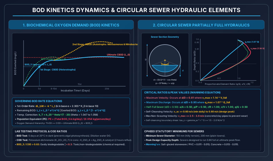
BOD Kinetics Dynamics & Circular Sewer Hydraulic Elements

4.1 Theoretical Oxygen Demand (ThOD)

The calculated stoichiometric mass of molecular oxygen (O2\text{O}_2) required to completely oxidize an organic compound of known chemical formula (CaHbOcNd\text{C}_a\text{H}_b\text{O}_c\text{N}_d) into CO2,H2O\text{CO}_2, \text{H}_2\text{O}, and NH3\text{NH}_3 (or fully oxidized NO3−\text{NO}_3^-):

CaHbOcNd+(a+b4−c2−3d4)O2→a CO2+(b−3d2)H2O+d NH3\text{C}_a\text{H}_b\text{O}_c\text{N}_d + \left(a + \frac{b}{4} - \frac{c}{2} - \frac{3d}{4}\right)\text{O}_2 \to a\,\text{CO}_2 + \left(\frac{b - 3d}{2}\right)\text{H}_2\text{O} + d\,\text{NH}_3

If nitrogen is further oxidized to nitrate:

NH3+2 O2→HNO3+H2O\text{NH}_3 + 2\,\text{O}_2 \to \text{HNO}_3 + \text{H}_2\text{O}

4.2 Chemical Oxygen Demand (COD)

A standard laboratory titration test measuring the oxygen equivalent of organic matter susceptible to chemical oxidation by a boiling mixture of potassium dichromate (K2Cr2O7\text{K}_2\text{Cr}_2\text{O}_7) in concentrated sulfuric acid (H2SO4\text{H}_2\text{SO}_4) in the presence of silver sulfate (Ag2SO4\text{Ag}_2\text{SO}_4, catalyst) and mercuric sulfate (HgSO4\text{HgSO}_4, suppresses chloride interference) over a 2-hour reflux period:

Cr2O72−+14 H++6 e−→2 Cr3++7 H2O\text{Cr}_2\text{O}_7^{2-} + 14\,\text{H}^+ + 6\,e^- \to 2\,\text{Cr}^{3+} + 7\,\text{H}_2\text{O}

Unreacted dichromate is back-titrated against ferrous ammonium sulfate (FAS) using ferroin indicator:

COD (mg/L)=(Vblank−Vsample)×NFAS×8000Vsample, mL\text{COD (mg/L)} = \frac{(V_{\text{blank}} - V_{\text{sample}}) \times N_{\text{FAS}} \times 8000}{V_{\text{sample, mL}}}

4.3 Total Organic Carbon (TOC)

Determined instrumental analysis wherein organic carbon is combusted catalytically at 680∘C−950∘C680^\circ\text{C} - 950^\circ\text{C} to CO2\text{CO}_2, which is quantified by an infrared gas analyzer.

4.4 Biodegradability Index & Demand Hierarchy

ThOD≥COD≥BODu>BOD5\text{ThOD} \ge \text{COD} \ge \text{BOD}_u > \text{BOD}_5
  • BOD5/COD>0.60\text{BOD}_5 / \text{COD} > 0.60: Highly biodegradable; amenable to conventional aerobic or anaerobic biological treatment without chemical conditioning.
  • 0.30≤BOD5/COD≤0.600.30 \le \text{BOD}_5 / \text{COD} \le 0.60: Moderately biodegradable; requires acclimated seed cultures or extended aeration.
  • BOD5/COD<0.30\text{BOD}_5 / \text{COD} < 0.30: Non-biodegradable or toxic; contains recalcitrant aromatics, synthetic polymers, or heavy metals; requires chemical oxidation (Fenton's, ozonation) or wet air oxidation.

5. First-Order BOD Kinetics & Temperature Corrections

5.1 First-Order Rate Formulation

The rate at which organic matter is biochemically decomposed by heterotrophic microorganisms is proportional to the concentration of unoxidized organic substrate remaining in the system:

dLtdt=−k⋅Lt(Base e)ordLtdt=−KD⋅Lt(Base 10)\frac{dL_t}{dt} = -k \cdot L_t \quad (\text{Base } e) \quad \text{or} \quad \frac{dL_t}{dt} = -K_D \cdot L_t \quad (\text{Base } 10)

Integrating from t=0t = 0 (Lt=L0L_t = L_0, ultimate carbonaceous BOD) to time tt:

Lt=L0⋅e−k⋅t=L0⋅10−KD⋅tL_t = L_0 \cdot e^{-k \cdot t} = L_0 \cdot 10^{-K_D \cdot t}

Where:

  • L0=L_0 = ultimate carbonaceous biochemical oxygen demand (mg/L\text{mg/L})
  • Lt=L_t = oxygen demand of organic matter remaining at time tt (mg/L\text{mg/L})
  • k=k = reaction rate constant to base ee (day−1\text{day}^{-1})
  • KD=K_D = reaction rate constant to base 1010 (day−1\text{day}^{-1}), where k=2.303×KDk = 2.303 \times K_D

The BOD exerted (consumed) by the microorganisms up to time tt (yty_t) is the difference between initial ultimate demand and remaining demand:

yt=L0−Lt=L0⋅(1−e−k⋅t)=L0⋅(1−10−KD⋅t)y_t = L_0 - L_t = L_0 \cdot \left(1 - e^{-k \cdot t}\right) = L_0 \cdot \left(1 - 10^{-K_D \cdot t}\right)

For typical municipal domestic sewage at 20∘C20^\circ\text{C}:

k20≈0.23 day−1(KD,20≈0.10 day−1)k_{20} \approx 0.23\text{ day}^{-1} \quad (K_{D,20} \approx 0.10\text{ day}^{-1}) y5=L0⋅(1−e−0.23×5)=L0⋅(1−e−1.15)=L0⋅(1−0.3166)=0.6834⋅L0≈68% of L0y_5 = L_0 \cdot \left(1 - e^{-0.23 \times 5}\right) = L_0 \cdot \left(1 - e^{-1.15}\right) = L_0 \cdot (1 - 0.3166) = 0.6834 \cdot L_0 \approx 68\% \text{ of } L_0

5.2 Temperature Dependence of BOD Rate Constant

Biological metabolic rates accelerate with rising temperature according to the van 't Hoff-Arrhenius relationship:

kT=k20⋅θ(T−20)k_T = k_{20} \cdot \theta^{(T - 20)}

Where:

  • θ=1.056\theta = 1.056 for temperature range 20∘C≤T≤30∘C20^\circ\text{C} \le T \le 30^\circ\text{C}
  • θ=1.135\theta = 1.135 for temperature range 4∘C≤T≤20∘C4^\circ\text{C} \le T \le 20^\circ\text{C}
  • In standard academic exam questions, θ=1.047\theta = 1.047 is frequently adopted across the entire range.
  • Crucial Physical Nuance: Temperature alters the speed (kk) of biological consumption, but does NOT alter the ultimate quantity of carbonaceous organic matter (L0L_0 remains constant regardless of temperature!).

5.3 Nitrogenous Biochemical Oxygen Demand (NBOD)

The aerobic decomposition of wastewater occurs in two distinct successive stages:

  1. First-Stage (Carbonaceous BOD / CBOD): Heterotrophic bacteria oxidize carbonaceous carbonaceous organic matter to CO2\text{CO}_2 and H2O\text{H}_2\text{O}. Commences immediately (t=0t = 0).
  2. Second-Stage (Nitrogenous BOD / NBOD): Autotrophic nitrifying bacteria oxidize ammonia nitrogen to nitrite and nitrate: 2 NH4++3 O2→Nitrosomonas2 NO2−+4 H++2 H2O2\,\text{NH}_4^+ + 3\,\text{O}_2 \xrightarrow{\text{Nitrosomonas}} 2\,\text{NO}_2^- + 4\,\text{H}^+ + 2\,\text{H}_2\text{O} 2 NO2−+O2→Nitrobacter2 NO3−2\,\text{NO}_2^- + \text{O}_2 \xrightarrow{\text{Nitrobacter}} 2\,\text{NO}_3^-
    • Total stoichiometric oxygen demand for nitrification: 1 mg of NH4+-N requires 4.57 mg of O2(64+1614=4.57)1\text{ mg of NH}_4^+\text{-N requires } 4.57\text{ mg of O}_2 \quad \left(\frac{64 + 16}{14} = 4.57\right)
    • Lag Period: Nitrifiers have a much lower maximum specific growth rate (μmax\mu_{\text{max}}) than heterotrophs. Consequently, NBOD exertion is suppressed and only manifests after 8 to 10 days8 \text{ to } 10\text{ days} of incubation at 20∘C20^\circ\text{C}.
    • The standard 5-day BOD test (BOD5\text{BOD}_5) isolates pure carbonaceous demand without NBOD interference.

5.4 Population Equivalent (PE)

Industrial and commercial wastewaters are normalized to an equivalent human contributing population based on per-capita daily 5-day BOD production:

Population Equivalent (PE)=Total Industrial BOD5 Load (kg/day)Per Capita Domestic BOD5 Contribution (kg/person/day)\text{Population Equivalent (PE)} = \frac{\text{Total Industrial BOD}_5 \text{ Load (kg/day)}}{\text{Per Capita Domestic BOD}_5 \text{ Contribution (kg/person/day)}}
  • CPHEEO Indian standard domestic contribution: 45−54 g/person/day45 - 54\text{ g/person/day} (0.045−0.054 kg/capita⋅day0.045 - 0.054\text{ kg/capita}\cdot\text{day}).
  • Western / US standard: 75−80 g/person/day75 - 80\text{ g/person/day} (0.075−0.080 kg/capita⋅day0.075 - 0.080\text{ kg/capita}\cdot\text{day}).

6. Sewerage Systems & Flow Estimation

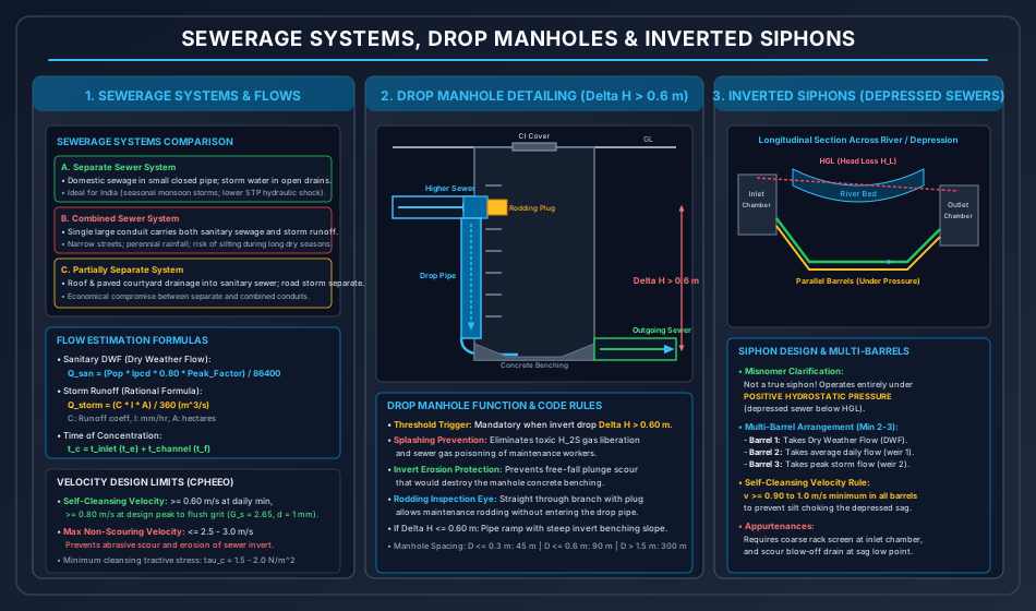
Sewerage Systems, Drop Manholes & Inverted Siphons

6.1 Sewerage Classification

  1. Separate System: Two independent conduit networks: (i) closed gravity sewers conveying domestic and industrial foul wastewater directly to the STP; (ii) open or closed stormwater drains discharging directly into watercourses.
    • Advantages: Uniform flow to STP; smaller sewer sizes; no large storm overflows.
    • Suitability: Subtropical monsoon climates with concentrated seasonal downpours (standard in India).
  2. Combined System: Single network conveying both sanitary sewage and urban stormwater runoff.
    • Advantages: Single pipe in narrow city rights-of-way; flushes sewer lines during rain.
    • Disadvantages: Huge diameters; risk of dry-season silting; heavy hydraulic shocks to STPs during storms requiring Combined Sewer Overflows (CSOs).
    • Suitability: Temperate regions with year-round, uniform precipitation.
  3. Partially Separate System: Sanitary sewers accept foul sewage plus drainage from residential roofs and courtyards, while street surface runoff flows in separate drains.

6.2 Dry Weather Flow (DWF) Estimation

Sanitary wastewater discharge is derived from municipal water consumption:

Qsan, avg=Population×qwater×ηsewerQ_{\text{san, avg}} = \text{Population} \times q_{\text{water}} \times \eta_{\text{sewer}}

Where:

  • qwater=q_{\text{water}} = per-capita water supply rate (135−200 lpcd135 - 200\text{ lpcd}).
  • ηsewer=\eta_{\text{sewer}} = sewage generation coefficient =0.75−0.85= 0.75 - 0.85 (typically taken as 0.800.80, meaning 80%80\% of supplied water appears as sewage).

Peak Factor Multipliers (CPHEEO Standards)

To accommodate diurnal morning and evening peak toilet and bath discharges:

Qsan, design=Qsan, avg×Peak FactorQ_{\text{san, design}} = Q_{\text{san, avg}} \times \text{Peak Factor}
Contributing Population CPHEEO Design Peak Factor
Up to 20,00020,000 3.003.00
20,00120,001 to 50,00050,000 2.502.50
50,00150,001 to 750,000750,000 2.252.25
Above 750,000750,000 2.002.00

6.3 Storm Sewage Estimation: Rational Formula

For catchments with area A≤50 km2A \le 50\text{ km}^2, the peak stormwater runoff discharge is governed by the Rational Equation:

Qp=1360⋅C⋅I⋅A(SI units: Qp in m3/s, I in mm/hr, A in hectares)Q_p = \frac{1}{360} \cdot C \cdot I \cdot A \quad (\text{SI units: } Q_p \text{ in m}^3/\text{s}, \, I \text{ in mm/hr}, \, A \text{ in hectares})

Where:

  • C=C = composite runoff coefficient (impervious asphalt/roofs =0.80−0.90= 0.80 - 0.90; lawns/parks =0.10−0.20= 0.10 - 0.20; composite residential =0.40−0.60= 0.40 - 0.60).
  • I=I = critical rainfall intensity (mm/hr\text{mm/hr}) corresponding to a duration equal to the time of concentration (tct_c).
  • tc=te+tft_c = t_e + t_f, where tet_e is inlet/overland entry time (5−15 min5 - 15\text{ min}) and tft_f is channel travel time (L/vL/v).

7. Hydraulics of Sewer Conduits Running Partially Full

7.1 Velocity Bounds & Tractive Shear Stress

Sewers operate under gravity as open channels. Unlike pressure water mains, sewers convey suspended inorganic grit (Gs≈2.65G_s \approx 2.65) and decomposing organic solids (Gs≈1.20G_s \approx 1.20).

1. Self-Cleansing Velocity (vscv_{\text{sc}})

The minimum velocity required to scour settled particles and prevent deposition:

  • At daily minimum flow: vmin≥0.60 m/sv_{\text{min}} \ge 0.60\text{ m/s}
  • At design peak daily flow: vpeak≥0.80 m/sv_{\text{peak}} \ge 0.80\text{ m/s}

Governed by Camp's adaptation of Shield's critical shear stress formulation:

vsc=8βg(Gs−1)dpf′=1nRH1/6τcγwv_{\text{sc}} = \sqrt{\frac{8 \beta g (G_s - 1) d_p}{f'}} = \frac{1}{n} R_H^{1/6} \sqrt{\frac{\tau_c}{\gamma_w}}

Where boundary critical shear stress τc=γwRHS≥1.5−2.0 N/m2\tau_c = \gamma_w R_H S \ge 1.5 - 2.0\text{ N/m}^2.

2. Maximum Non-Scouring Velocity (vmaxv_{\text{max}})

To eliminate severe abrasive erosion of the sewer pipe invert by rolling quartz sand and gravel:

  • Glazed vitrified stoneware pipes: ≤3.0 m/s\le 3.0\text{ m/s}
  • Cast-in-situ plain cement concrete / RCC pipes: ≤2.5−3.0 m/s\le 2.5 - 3.0\text{ m/s}
  • Cast Iron / Ductile Iron pipes: ≤4.5 m/s\le 4.5\text{ m/s}

7.2 Geometric Elements of Circular Conduits Running Partially Full

Let DD be the internal diameter of the sewer and dd be the partial depth of flow. The cross-section subtends an angle 2θ2\theta at the pipe center (in radians).

          /-------\
         /    ^    \
        |     |     |
        |   (2*theta)|
        |     v     |
        \   ~~~~~   /  <-- Water surface (depth d)
         \_________/
  1. Depth of Flow (dd): cos⁡θ=1−2dD  ⟹  d=D2(1−cos⁡θ)\cos\theta = 1 - \frac{2d}{D} \implies d = \frac{D}{2}(1 - \cos\theta)
  2. Wetted Area (aa): a=D28(2θ−sin⁡2θ)a = \frac{D^2}{8}(2\theta - \sin 2\theta) Full Area: A=π4D2A = \frac{\pi}{4} D^2.
  3. Wetted Perimeter (pp): p=D⋅θ(θ in radians)p = D \cdot \theta \quad (\theta \text{ in radians}) Full Perimeter: P=πDP = \pi D.
  4. Hydraulic Radius (rr): r=ap=D28(2θ−sin⁡2θ)D⋅θ=D4(1−sin⁡2θ2θ)r = \frac{a}{p} = \frac{\frac{D^2}{8}(2\theta - \sin 2\theta)}{D \cdot \theta} = \frac{D}{4}\left(1 - \frac{\sin 2\theta}{2\theta}\right) Full Hydraulic Radius: R=D4R = \frac{D}{4}.

7.3 Hydraulic Elements Ratios (Manning's Equation)

Assuming Manning's roughness coefficient nn is independent of depth (n=N=constn = N = \text{const}):

vV=(rR)2/3=(1−sin⁡2θ2θ)2/3\frac{v}{V} = \left(\frac{r}{R}\right)^{2/3} = \left(1 - \frac{\sin 2\theta}{2\theta}\right)^{2/3} qQ=(aA)⋅(vV)=[2θ−sin⁡2θ2π]⋅(1−sin⁡2θ2θ)2/3\frac{q}{Q} = \left(\frac{a}{A}\right) \cdot \left(\frac{v}{V}\right) = \left[\frac{2\theta - \sin 2\theta}{2\pi}\right] \cdot \left(1 - \frac{\sin 2\theta}{2\theta}\right)^{2/3}

Critical Hydraulic Landmarks

  1. Half-Full Condition (d/D=0.50, θ=π/2d/D = 0.50, \, \theta = \pi/2): aA=0.50,pP=0.50,rR=1.00,vV=1.00,qQ=0.50\frac{a}{A} = 0.50, \quad \frac{p}{P} = 0.50, \quad \frac{r}{R} = 1.00, \quad \frac{v}{V} = 1.00, \quad \frac{q}{Q} = 0.50 Crucial Exam Fact: A circular sewer running half-full possesses the identical velocity as when running completely full!
  2. Maximum Velocity Condition (d/D=0.81d/D = 0.81):
    • Subtended angle: 2θ≈257.5∘=4.494 rad2\theta \approx 257.5^\circ = 4.494\text{ rad}.
    • Relative velocity reaches a maximum: (vV)max=1.14(14% higher than full velocity!)\left(\frac{v}{V}\right)_{\text{max}} = 1.14 \quad (14\% \text{ higher than full velocity!})
    • Physical Mechanism: As the water level rises past 0.81D0.81 D, the top perimeter of the pipe increases the drag surface area (pp) much faster than the incremental cross-sectional flow area (aa), causing hydraulic radius (r=a/pr = a/p) and velocity to diminish.
  3. Maximum Discharge Condition (d/D=0.95d/D = 0.95):
    • Subtended angle: 2θ≈308∘=5.375 rad2\theta \approx 308^\circ = 5.375\text{ rad}.
    • Relative discharge reaches a maximum: (qQ)max=1.07(7% higher than full pipe discharge!)\left(\frac{q}{Q}\right)_{\text{max}} = 1.07 \quad (7\% \text{ higher than full pipe discharge!})
    • Above 0.95D0.95 D, air surface tension resistance is replaced by wall friction over the remaining crown, throttling total capacity.

8. Sewer Appurtenances & Ancillary Structures

8.1 Manholes

Masonry or reinforced concrete inspection chambers constructed along sewer alignments to provide access for inspection, cleaning, rodding, and maintenance.

  • Locations: Mandatory at all changes in sewer diameter, alignment (bends), bed gradient, and pipe junctions, as well as along straight runs at statutory intervals.
  • CPHEEO Spacing Standards:
    • Pipe diameter D≤300 mmD \le 300\text{ mm}: Maximum spacing 45 m45\text{ m}
    • 301 to 500 mm301\text{ to } 500\text{ mm}: Maximum spacing 75 m75\text{ m}
    • 501 to 900 mm501\text{ to } 900\text{ mm}: Maximum spacing 90 m90\text{ m}
    • 901 to 1200 mm901\text{ to } 1200\text{ mm}: Maximum spacing 120 m120\text{ m}
    • D>1500 mmD > 1500\text{ mm}: Spacing up to 300 m300\text{ m}
  • Depth Classification:
    • Shallow Manhole: Depth 0.75−0.90 m0.75 - 0.90\text{ m} (at the start of a branch sewer).
    • Normal Manhole: Depth 0.90−1.50 m0.90 - 1.50\text{ m}.
    • Deep Manhole: Depth >1.50 m> 1.50\text{ m} (requires access ladder and heavy-duty cast iron frame).

8.2 Drop Manholes

A specialized manhole constructed when a branch sewer enters an existing or main sewer at an elevation significantly higher than the main sewer invert.

  • Statutory Threshold: Mandatory whenever the difference in invert levels between the incoming branch sewer and the outgoing sewer exceeds 0.60 m0.60\text{ m} (600 mm600\text{ mm}).
  • Structural Configuration:
    • A vertical pipe (cast iron or ductile iron) is connected to the incoming sewer immediately outside the manhole chamber.
    • At the top of the vertical drop, a tee-junction is provided with a horizontal inspection branch projecting into the manhole, sealed with a removable rodding plug to allow straight-line maintenance clearing.
    • At the base of the drop pipe, a 90∘90^\circ duckfoot bend discharges smoothly along the concrete invert benching channel in the direction of downstream flow.
  • Engineering Necessity:
    1. Prevents free sewage cascading and splashing inside the manhole shaft.
    2. Splashing strips toxic hydrogen sulfide (H2S\text{H}_2\text{S}) and methane (CH4\text{CH}_4) from the liquid, posing lethal asphyxiation hazards to workers.
    3. Eliminates severe hydraulic plunge impact that would disintegrate the brick masonry walls and concrete benching.
    4. If ΔH≤0.60 m\Delta H \le 0.60\text{ m}, a drop pipe is omitted; instead, the sewage is guided down an inclined ramp formed in the concrete benching.

8.3 Inverted Siphons (Depressed Sewers / Sag Pipes)

An inverted siphon is a section of sewer that drops below the hydraulic grade line to traverse an obstruction (such as a river, depressed railway cutting, highway underpass, or subway tunnel) and rises back up to the normal gravity sewer grade.

  • Hydraulic Nature: Despite the name, an inverted siphon is NOT a true vacuum siphon. It is a depressed sewer flowing full under positive hydrostatic pressure head.
  • Multi-Barrel Requirement (Minimum 2 to 3 Parallel Barrels):
    • Because flow varies dramatically between dry weather flow (DWF) and peak wet weather flow, a single large pipe would experience critically low velocities during dry seasons, causing grit deposition in the depressed sag.
    • Inlet Distribution Chamber: Fitted with overflow weirs of varying crest elevations:
      • Barrel 1 (Smallest): Sized for Dry Weather Flow (DWF) with minimum velocity v≥0.90−1.0 m/sv \ge 0.90 - 1.0\text{ m/s}.
      • Barrel 2: Sized for average daily flow, brought into operation as water spills over Weir 1.
      • Barrel 3: Sized for peak storm flow, engaged over Weir 2 during severe downpours.
  • Self-Cleansing Velocity Rule: Invert barrels must achieve v≥1.0 m/sv \ge 1.0\text{ m/s} at least once daily to prevent silt accumulation.

9. Step-by-Step Analytical Derivations

9.1 Derivation of First-Order BOD Exertion Equation

Let LtL_t represent the concentration of carbonaceous organic matter remaining at time tt, expressed as ultimate oxygen demand equivalent (mg/L\text{mg/L}).
Assuming the rate of biochemical oxidation by heterotrophic microorganisms is a first-order reaction with respect to remaining substrate:

dLtdt=−k⋅Lt(1)\frac{dL_t}{dt} = -k \cdot L_t \tag{1}

Separating variables:

dLtLt=−k⋅dt(2)\frac{dL_t}{L_t} = -k \cdot dt \tag{2}

Integrating both sides from t=0t = 0 (where initial ultimate organic matter is L0L_0) to time tt (where organic matter remaining is LtL_t):

∫L0LtdLtLt=−k∫0tdt(3)\int_{L_0}^{L_t} \frac{dL_t}{L_t} = -k \int_{0}^{t} dt \tag{3} ln⁡(LtL0)=−k⋅t(4)\ln\left(\frac{L_t}{L_0}\right) = -k \cdot t \tag{4}

Taking the exponential on both sides:

LtL0=e−k⋅t  ⟹  Lt=L0⋅e−k⋅t(5)\frac{L_t}{L_0} = e^{-k \cdot t} \implies L_t = L_0 \cdot e^{-k \cdot t} \tag{5}

The biochemical oxygen demand exerted (consumed) up to time tt, designated as yty_t, represents the initial organic matter oxidized:

yt=L0−Lt(6)y_t = L_0 - L_t \tag{6}

Substituting Eq. (5) into Eq. (6):

yt=L0−L0⋅e−k⋅t=L0(1−e−k⋅t)(7)y_t = L_0 - L_0 \cdot e^{-k \cdot t} = L_0 \left(1 - e^{-k \cdot t}\right) \tag{7}

Converting to base 10 where k=2.303×KDk = 2.303 \times K_D:

yt=L0(1−10−KD⋅t)■y_t = L_0 \left(1 - 10^{-K_D \cdot t}\right) \quad \blacksquare

9.2 Derivation of Circular Sewer Hydraulic Properties (a,p,ra, p, r)

Consider a circular sewer of internal diameter DD (radius R0=D/2R_0 = D/2) running partially full at liquid depth dd. Let 2θ2\theta be the angle subtended by the free water surface chord at the pipe center (in radians).

          O (Center)
         /|\
     R_0/ | \ R_0
       /__|__\
      A   M   B     (Chord AB = Top Width T)
        \ | /
         \|/
          C (Invert, Depth d = MC)
  1. Depth Formulation: In ΔOMA\Delta OMA, OM=R0cos⁡θOM = R_0 \cos\theta. The depth of flow dd is:

    d=R0−OM=R0−R0cos⁡θ=R0(1−cos⁡θ)=D2(1−cos⁡θ)(1)d = R_0 - OM = R_0 - R_0 \cos\theta = R_0(1 - \cos\theta) = \frac{D}{2}(1 - \cos\theta) \tag{1}
  2. Wetted Area Formulation (aa): The wetted area aa equals the area of the circular sector OACBOACB minus the area of the triangle OABOAB:

    Area of Sector OACB=12R02(2θ)=R02θ=D24θ\text{Area of Sector } OACB = \frac{1}{2} R_0^2 (2\theta) = R_0^2 \theta = \frac{D^2}{4}\theta Area of Triangle OAB=12⋅Base⋅Height=12(2R0sin⁡θ)(R0cos⁡θ)=R02sin⁡θcos⁡θ=R022sin⁡2θ=D28sin⁡2θ\text{Area of Triangle } OAB = \frac{1}{2} \cdot \text{Base} \cdot \text{Height} = \frac{1}{2} (2 R_0 \sin\theta)(R_0 \cos\theta) = R_0^2 \sin\theta\cos\theta = \frac{R_0^2}{2}\sin 2\theta = \frac{D^2}{8}\sin 2\theta a=D24θ−D28sin⁡2θ=D28(2θ−sin⁡2θ)(2)a = \frac{D^2}{4}\theta - \frac{D^2}{8}\sin 2\theta = \frac{D^2}{8}(2\theta - \sin 2\theta) \tag{2}
  3. Wetted Perimeter (pp): The arc length along the bottom boundary contacting the fluid:

    p=R0(2θ)=(D2)(2θ)=D⋅θ(3)p = R_0 (2\theta) = \left(\frac{D}{2}\right)(2\theta) = D \cdot \theta \tag{3}
  4. Hydraulic Radius (rr):

    r=ap=D28(2θ−sin⁡2θ)D⋅θ=D8θ(2θ−sin⁡2θ)=D4(1−sin⁡2θ2θ)■(4)r = \frac{a}{p} = \frac{\frac{D^2}{8}(2\theta - \sin 2\theta)}{D \cdot \theta} = \frac{D}{8\theta}(2\theta - \sin 2\theta) = \frac{D}{4}\left(1 - \frac{\sin 2\theta}{2\theta}\right) \quad \blacksquare \tag{4}

9.3 Proof that Maximum Flow Velocity Occurs at d/D≈0.81d/D \approx 0.81

According to Manning's equation for open channel flow with constant bed slope SS and roughness nn:

v=1nr2/3S1/2v = \frac{1}{n} r^{2/3} S^{1/2}

Since nn and SS are constant, velocity vv is maximized when hydraulic radius rr is maximized:

dvdθ=0  ⟺  drdθ=0(1)\frac{dv}{d\theta} = 0 \iff \frac{dr}{d\theta} = 0 \tag{1}

From Eq. (4) of Section 9.2:

r(θ)=D4(1−sin⁡2θ2θ)r(\theta) = \frac{D}{4}\left(1 - \frac{\sin 2\theta}{2\theta}\right)

Differentiating r(θ)r(\theta) with respect to θ\theta:

drdθ=D4[−(2θ)(2cos⁡2θ)−(sin⁡2θ)(2)(2θ)2]=0\frac{dr}{d\theta} = \frac{D}{4} \left[ -\frac{(2\theta)(2\cos 2\theta) - (\sin 2\theta)(2)}{(2\theta)^2} \right] = 0 (2θ)(2cos⁡2θ)−2sin⁡2θ=0(2\theta)(2\cos 2\theta) - 2\sin 2\theta = 0 2θcos⁡2θ=sin⁡2θ  ⟹  tan⁡2θ=2θ(2)2\theta \cos 2\theta = \sin 2\theta \implies \tan 2\theta = 2\theta \tag{2}

Solving the transcendental equation tan⁡(2θ)=2θ\tan(2\theta) = 2\theta numerically for the non-trivial roots in the range π<2θ<2π\pi < 2\theta < 2\pi:

2θ=4.4934 rad≈257.45∘(3)2\theta = 4.4934\text{ rad} \approx 257.45^\circ \tag{3}

Using the depth relation from Eq. (1):

θ=257.45∘2=128.73∘\theta = \frac{257.45^\circ}{2} = 128.73^\circ dD=12(1−cos⁡θ)=12(1−cos⁡128.73∘)=12(1−(−0.6256))=1.62562=0.8128≈0.81■(4)\frac{d}{D} = \frac{1}{2}(1 - \cos\theta) = \frac{1}{2}(1 - \cos 128.73^\circ) = \frac{1}{2}(1 - (-0.6256)) = \frac{1.6256}{2} = 0.8128 \approx 0.81 \quad \blacksquare \tag{4}

Evaluating relative velocity ratio at 2θ=4.4934 rad2\theta = 4.4934\text{ rad}:

rR=1−sin⁡(4.4934)4.4934=1−−0.97654.4934=1+0.2173=1.2173\frac{r}{R} = 1 - \frac{\sin(4.4934)}{4.4934} = 1 - \frac{-0.9765}{4.4934} = 1 + 0.2173 = 1.2173 vmaxV=(rR)2/3=(1.2173)2/3=1.1396≈1.14■\frac{v_{\text{max}}}{V} = \left(\frac{r}{R}\right)^{2/3} = (1.2173)^{2/3} = 1.1396 \approx 1.14 \quad \blacksquare

10. Solved Numerical Example 1: BOD Kinetics & Population Equivalent

Problem Statement

A composite municipal wastewater sample collected from an urban drainage district has a 5-day Biochemical Oxygen Demand (BOD5\text{BOD}_5) of 180.0 mg/L180.0\text{ mg/L} when incubated at 20∘C20^\circ\text{C}.
Laboratory analysis established that the first-order reaction rate constant (to base ee) is k20=0.230 day−1k_{20} = 0.230\text{ day}^{-1}.

  1. Calculate the ultimate carbonaceous biochemical oxygen demand (L0L_0) of the wastewater.
  2. Determine the reaction rate constant at 27∘C27^\circ\text{C} (k27k_{27}) assuming temperature coefficient θ=1.047\theta = 1.047.
  3. Compute the 3-day BOD exerted by the wastewater at 27∘C27^\circ\text{C} (y3,27y_{3,27}).
  4. If the municipal district generates an average wastewater discharge of 40.0 MLD40.0\text{ MLD} (40,000 m3/day40,000\text{ m}^3/\text{day}), calculate the total daily BOD5\text{BOD}_5 load in kg/day\text{kg/day}.
  5. Determine the Population Equivalent (PE) of the discharge based on standard per-capita BOD production of 54.0 g BOD5/person⋅day54.0\text{ g BOD}_5/\text{person}\cdot\text{day}.

Complete Analytical Solution

1. Ultimate Carbonaceous BOD (L0L_0)

Using the first-order exertion equation:

yt=L0(1−e−k⋅t)y_t = L_0 \left(1 - e^{-k \cdot t}\right)

For t=5 dayst = 5\text{ days}, T=20∘CT = 20^\circ\text{C}, y5=180.0 mg/Ly_5 = 180.0\text{ mg/L}, and k20=0.230 day−1k_{20} = 0.230\text{ day}^{-1}:

k20⋅t=0.230×5=1.150k_{20} \cdot t = 0.230 \times 5 = 1.150 e−1.150=0.316637e^{-1.150} = 0.316637 1−e−1.150=1−0.316637=0.6833631 - e^{-1.150} = 1 - 0.316637 = 0.683363

Solving for L0L_0:

L0=y51−e−k20⋅5=180.00.683363=263.403 mg/L≈263.40 mg/LL_0 = \frac{y_5}{1 - e^{-k_{20} \cdot 5}} = \frac{180.0}{0.683363} = 263.403\text{ mg/L} \approx 263.40\text{ mg/L}

2. Reaction Rate Constant at 27∘C27^\circ\text{C} (k27k_{27})

Applying the Arrhenius temperature correction with θ=1.047\theta = 1.047:

k27=k20⋅θ(27−20)=0.230×(1.047)7k_{27} = k_{20} \cdot \theta^{(27 - 20)} = 0.230 \times (1.047)^7 (1.047)7=1.37905(1.047)^7 = 1.37905 k27=0.230×1.37905=0.31718 day−1≈0.3172 day−1k_{27} = 0.230 \times 1.37905 = 0.31718\text{ day}^{-1} \approx 0.3172\text{ day}^{-1}

3. 3-Day BOD Exerted at 27∘C27^\circ\text{C} (y3,27y_{3,27})

y3,27=L0(1−e−k27⋅3)y_{3,27} = L_0 \left(1 - e^{-k_{27} \cdot 3}\right)

Note that L0L_0 remains invariant with temperature (L0=263.403 mg/LL_0 = 263.403\text{ mg/L}):

k27⋅3=0.31718×3=0.95154k_{27} \cdot 3 = 0.31718 \times 3 = 0.95154 e−0.95154=0.386144e^{-0.95154} = 0.386144 1−e−0.95154=1−0.386144=0.6138561 - e^{-0.95154} = 1 - 0.386144 = 0.613856 y3,27=263.403×0.613856=161.702 mg/L≈161.70 mg/Ly_{3,27} = 263.403 \times 0.613856 = 161.702\text{ mg/L} \approx 161.70\text{ mg/L}

4. Total Daily BOD5\text{BOD}_5 Load

Discharge Q=40.0 MLD=40,000 m3/dayQ = 40.0\text{ MLD} = 40,000\text{ m}^3/\text{day}.

Total Daily BOD5=Q×BOD5=40,000 m3/day×180.0 g/m3=7,200,000 g/day=7,200.0 kg/day\text{Total Daily BOD}_5 = Q \times \text{BOD}_5 = 40,000\text{ m}^3/\text{day} \times 180.0\text{ g/m}^3 = 7,200,000\text{ g/day} = 7,200.0\text{ kg/day}

5. Population Equivalent (PE)

Standard per-capita daily load =54.0 g/person⋅day=0.054 kg/person⋅day= 54.0\text{ g/person}\cdot\text{day} = 0.054\text{ kg/person}\cdot\text{day}.

PE=Total Daily LoadPer-Capita Load=7,200.0 kg/day0.054 kg/person/day=133,333.3≈133,333 persons\text{PE} = \frac{\text{Total Daily Load}}{\text{Per-Capita Load}} = \frac{7,200.0\text{ kg/day}}{0.054\text{ kg/person/day}} = 133,333.3 \approx 133,333\text{ persons}

11. Solved Numerical Example 2: Circular Sewer Hydraulics Running Partially Full

Problem Statement

A circular precast concrete sewer pipe (n=0.013n = 0.013) has an internal diameter of D=900 mmD = 900\text{ mm} (0.90 m0.90\text{ m}) and is laid on a longitudinal bed slope of S=1 in 1000S = 1 \text{ in } 1000 (S=0.001S = 0.001).

  1. Calculate the flow velocity (VV) and volumetric discharge (QQ) when the sewer is flowing completely full under gravity.
  2. Determine the subtended angle 2θ2\theta, wetted area aa, wetted perimeter pp, and hydraulic radius rr when the sewer flows partially full at a depth of d=360 mmd = 360\text{ mm} (d/D=0.40d/D = 0.40).
  3. Calculate the flow velocity (vv) and discharge (qq) under this partially full depth (d=360 mmd = 360\text{ mm}).
  4. Check whether the self-cleansing velocity requirement (v≥0.60 m/sv \ge 0.60\text{ m/s}) is satisfied.

Complete Analytical Solution

1. Full Running Hydraulic Elements (Vfull,QfullV_{\text{full}}, Q_{\text{full}})

D=0.90 m,n=0.013,S=0.001D = 0.90\text{ m}, \quad n = 0.013, \quad S = 0.001 Afull=π4D2=π4(0.90)2=0.63617 m2A_{\text{full}} = \frac{\pi}{4} D^2 = \frac{\pi}{4} (0.90)^2 = 0.63617\text{ m}^2 Pfull=πD=π×0.90=2.82743 mP_{\text{full}} = \pi D = \pi \times 0.90 = 2.82743\text{ m} Rfull=D4=0.904=0.2250 mR_{\text{full}} = \frac{D}{4} = \frac{0.90}{4} = 0.2250\text{ m}

Using Manning's equation:

Vfull=1nRfull2/3S1/2=10.013×(0.2250)2/3×(0.001)1/2V_{\text{full}} = \frac{1}{n} R_{\text{full}}^{2/3} S^{1/2} = \frac{1}{0.013} \times (0.2250)^{2/3} \times (0.001)^{1/2} (0.2250)2/3=0.36993,0.001=0.0316228(0.2250)^{2/3} = 0.36993, \quad \sqrt{0.001} = 0.0316228 Vfull=0.36993×0.03162280.013=0.01169830.013=0.89987 m/s≈0.900 m/sV_{\text{full}} = \frac{0.36993 \times 0.0316228}{0.013} = \frac{0.0116983}{0.013} = 0.89987\text{ m/s} \approx 0.900\text{ m/s} Qfull=Afull×Vfull=0.63617×0.89987=0.57247 m3/s=572.47 L/sQ_{\text{full}} = A_{\text{full}} \times V_{\text{full}} = 0.63617 \times 0.89987 = 0.57247\text{ m}^3/\text{s} = 572.47\text{ L/s}

2. Geometric Elements at d=0.360 md = 0.360\text{ m} (d/D=0.40d/D = 0.40)

cos⁡θ=1−2(dD)=1−2(0.40)=1−0.80=0.200\cos\theta = 1 - 2\left(\frac{d}{D}\right) = 1 - 2(0.40) = 1 - 0.80 = 0.200 θ=arccos⁡(0.200)=1.36944 rad=78.463∘\theta = \arccos(0.200) = 1.36944\text{ rad} = 78.463^\circ 2θ=2×1.36944=2.73888 rad=156.926∘2\theta = 2 \times 1.36944 = 2.73888\text{ rad} = 156.926^\circ sin⁡(2θ)=sin⁡(156.926∘)=0.39192\sin(2\theta) = \sin(156.926^\circ) = 0.39192
  • Wetted Area (aa):

    a=D28(2θ−sin⁡2θ)=(0.90)28(2.73888−0.39192)=0.818×2.34696=0.23763 m2a = \frac{D^2}{8}(2\theta - \sin 2\theta) = \frac{(0.90)^2}{8} (2.73888 - 0.39192) = \frac{0.81}{8} \times 2.34696 = 0.23763\text{ m}^2 aAfull=0.237630.63617=0.3735(37.35% of full area)\frac{a}{A_{\text{full}}} = \frac{0.23763}{0.63617} = 0.3735 \quad (37.35\% \text{ of full area})
  • Wetted Perimeter (pp):

    p=D⋅θ=0.90×1.36944=1.23250 mp = D \cdot \theta = 0.90 \times 1.36944 = 1.23250\text{ m} pPfull=1.232502.82743=0.4359(43.59% of full perimeter)\frac{p}{P_{\text{full}}} = \frac{1.23250}{2.82743} = 0.4359 \quad (43.59\% \text{ of full perimeter})
  • Hydraulic Radius (rr):

    r=ap=0.237631.23250=0.19280 mr = \frac{a}{p} = \frac{0.23763}{1.23250} = 0.19280\text{ m} rRfull=0.192800.2250=0.8569(85.69% of full hydraulic radius)\frac{r}{R_{\text{full}}} = \frac{0.19280}{0.2250} = 0.8569 \quad (85.69\% \text{ of full hydraulic radius})

3. Partially Full Velocity (vv) & Discharge (qq)

v=1nr2/3S1/2=10.013×(0.19280)2/3×0.001v = \frac{1}{n} r^{2/3} S^{1/2} = \frac{1}{0.013} \times (0.19280)^{2/3} \times \sqrt{0.001} (0.19280)2/3=0.33371(0.19280)^{2/3} = 0.33371 v=0.33371×0.03162280.013=0.81177 m/s≈0.812 m/sv = \frac{0.33371 \times 0.0316228}{0.013} = 0.81177\text{ m/s} \approx 0.812\text{ m/s} vVfull=0.811770.89987=0.9021(90.21% of full velocity)\frac{v}{V_{\text{full}}} = \frac{0.81177}{0.89987} = 0.9021 \quad (90.21\% \text{ of full velocity}) q=a×v=0.23763 m2×0.81177 m/s=0.19290 m3/s=192.90 L/sq = a \times v = 0.23763\text{ m}^2 \times 0.81177\text{ m/s} = 0.19290\text{ m}^3/\text{s} = 192.90\text{ L/s} qQfull=0.192900.57247=0.3370(33.70% of full discharge)\frac{q}{Q_{\text{full}}} = \frac{0.19290}{0.57247} = 0.3370 \quad (33.70\% \text{ of full discharge})

4. Self-Cleansing Velocity Evaluation

v=0.812 m/s≥0.60 m/sv = 0.812\text{ m/s} \ge 0.60\text{ m/s}

The velocity comfortably exceeds the minimum threshold of 0.60 m/s0.60\text{ m/s} (and matches design peak 0.80 m/s0.80\text{ m/s}), ensuring that no solid particles, sand, or grease settle at d/D=0.40d/D = 0.40.


12. Solved Numerical Example 3: Combined Sewer Design & Rational Runoff

Problem Statement

A planned municipal drainage district has an area of A=50.0 hectaresA = 50.0\text{ hectares} with a composite catchment runoff coefficient C=0.45C = 0.45.
The intensity-duration relationship for a 5-year design frequency storm in this region is:

I=750tc+10(where I is in mm/hr and tc is in minutes)I = \frac{750}{t_c + 10} \quad (\text{where } I \text{ is in mm/hr and } t_c \text{ is in minutes})

The estimated time of concentration of the drainage basin is tc=20 minutest_c = 20\text{ minutes}.

The district supports a residential population of 40,00040,000 persons with an average domestic water supply rate of 150.0 lpcd150.0\text{ lpcd}.
Assuming 80%80\% of domestic water is converted into sanitary wastewater and the design peak factor for sanitary sewage is 2.502.50:

  1. Calculate the design storm runoff discharge (QstormQ_{\text{storm}}) via the Rational Formula.
  2. Determine the average sanitary sewage flow (Qsan, avgQ_{\text{san, avg}}) and design peak sanitary flow (Qsan, peakQ_{\text{san, peak}}).
  3. Compute the total design combined discharge (QcombinedQ_{\text{combined}}).
  4. Determine the required internal diameter (DD) of a circular precast concrete combined sewer (n=0.013n = 0.013) running completely full on a longitudinal slope of S=1 in 800S = 1 \text{ in } 800 (0.001250.00125).

Complete Analytical Solution

1. Design Storm Runoff Discharge (QstormQ_{\text{storm}})

tc=20 min  ⟹  I=75020+10=75030=25.00 mm/hrt_c = 20\text{ min} \implies I = \frac{750}{20 + 10} = \frac{750}{30} = 25.00\text{ mm/hr}

Using the Rational Equation:

Qstorm=1360⋅C⋅I⋅A=0.45×25.00×50.0360=562.5360=1.5625 m3/sQ_{\text{storm}} = \frac{1}{360} \cdot C \cdot I \cdot A = \frac{0.45 \times 25.00 \times 50.0}{360} = \frac{562.5}{360} = 1.5625\text{ m}^3/\text{s}

2. Sanitary Sewage Flow Estimation

Population=40,000,qwater=150.0 lpcd,ηsewer=0.80\text{Population} = 40,000, \quad q_{\text{water}} = 150.0\text{ lpcd}, \quad \eta_{\text{sewer}} = 0.80 Daily Total Domestic Sewage=40,000×150.0×0.80=4,800,000 L/day=4,800.0 m3/day\text{Daily Total Domestic Sewage} = 40,000 \times 150.0 \times 0.80 = 4,800,000\text{ L/day} = 4,800.0\text{ m}^3/\text{day}

Average sanitary discharge:

Qsan, avg=4,800.0 m386,400 s=0.05556 m3/s=55.56 L/sQ_{\text{san, avg}} = \frac{4,800.0\text{ m}^3}{86,400\text{ s}} = 0.05556\text{ m}^3/\text{s} = 55.56\text{ L/s}

With design peak factor =2.50= 2.50:

Qsan, peak=2.50×0.05556 m3/s=0.13889 m3/s=138.89 L/sQ_{\text{san, peak}} = 2.50 \times 0.05556\text{ m}^3/\text{s} = 0.13889\text{ m}^3/\text{s} = 138.89\text{ L/s}

3. Total Combined Design Flow (QcombinedQ_{\text{combined}})

Qcombined=Qstorm+Qsan, peak=1.5625+0.13889=1.70139 m3/s≈1.7014 m3/sQ_{\text{combined}} = Q_{\text{storm}} + Q_{\text{san, peak}} = 1.5625 + 0.13889 = 1.70139\text{ m}^3/\text{s} \approx 1.7014\text{ m}^3/\text{s}

(Observation: Storm runoff constitutes 91.8%91.8\% of the combined capacity!)

4. Required Diameter of Circular Sewer

Using Manning's equation for a circular conduit running full (A=π4D2,R=D4A = \frac{\pi}{4} D^2, R = \frac{D}{4}):

Q=A⋅1nR2/3S1/2=(π4D2)1n(D4)2/3S1/2Q = A \cdot \frac{1}{n} R^{2/3} S^{1/2} = \left(\frac{\pi}{4} D^2\right) \frac{1}{n} \left(\frac{D}{4}\right)^{2/3} S^{1/2} Q=π4×42/3⋅1n⋅S1/2⋅D8/3=π4×2.51984⋅S1/2n⋅D8/3=0.31168⋅S1/2n⋅D8/3Q = \frac{\pi}{4 \times 4^{2/3}} \cdot \frac{1}{n} \cdot S^{1/2} \cdot D^{8/3} = \frac{\pi}{4 \times 2.51984} \cdot \frac{S^{1/2}}{n} \cdot D^{8/3} = 0.31168 \cdot \frac{S^{1/2}}{n} \cdot D^{8/3}

Given S=1/800=0.00125  ⟹  S=0.035355S = 1/800 = 0.00125 \implies \sqrt{S} = 0.035355, and n=0.013n = 0.013:

Q=0.31168×0.0353550.013×D8/3=0.31168×2.71964×D8/3=0.84766⋅D8/3Q = 0.31168 \times \frac{0.035355}{0.013} \times D^{8/3} = 0.31168 \times 2.71964 \times D^{8/3} = 0.84766 \cdot D^{8/3}

Equating to Qcombined=1.70139 m3/sQ_{\text{combined}} = 1.70139\text{ m}^3/\text{s}:

0.84766⋅D8/3=1.701390.84766 \cdot D^{8/3} = 1.70139 D8/3=1.701390.84766=2.00716D^{8/3} = \frac{1.70139}{0.84766} = 2.00716 D=(2.00716)3/8=(2.00716)0.375=1.2986 m≈1,299 mmD = (2.00716)^{3/8} = (2.00716)^{0.375} = 1.2986\text{ m} \approx 1,299\text{ mm}

Design Recommendation: Adopt a standard commercial diameter of D=1,400 mmD = 1,400\text{ mm} (1.40 m1.40\text{ m}), allowing the sewer to flow at approximately d/D≈0.80d/D \approx 0.80 under design combined peak flow.


13. Common Misconceptions & Exam Traps

[!WARNING] Trap 1: Base ee vs Base 10 BOD Rate Constants
In competitive exams, check whether the rate constant is given as kk (Napierian / Base ee) or KDK_D (Common / Base 10). They differ by a factor of 2.3032.303:

k=2.303×KD(k20≈0.23 d−1  ⟺  KD,20≈0.10 d−1)k = 2.303 \times K_D \quad (k_{20} \approx 0.23\text{ d}^{-1} \iff K_{D,20} \approx 0.10\text{ d}^{-1})

Using kk inside 10−kt10^{-k t} or KDK_D inside e−KDte^{-K_D t} produces erroneous BOD values.

[!WARNING] Trap 2: Nitrogenous BOD in Standard 5-Day Test
Candidates often wonder why NBOD is omitted in standard BOD5\text{BOD}_5. Because nitrifying autotrophs (Nitrosomonas and Nitrobacter) have slow reproduction rates, nitrification begins only after 8 to 10 days8 \text{ to } 10\text{ days} at 20∘C20^\circ\text{C}. Thus, standard BOD5\text{BOD}_5 measures only Carbonaceous BOD (CBOD). If an uninhibited sample is incubated for 20 days, nitrification produces a second upward inflection in the exertion curve.

[!CAUTION] Trap 3: Maximum Velocity vs Maximum Discharge Depths
Candidates routinely invert these two landmarks:

  • Maximum velocity occurs at d/D=0.81d/D = 0.81 (vmax=1.14Vv_{\text{max}} = 1.14 V).
  • Maximum discharge occurs at d/D=0.95d/D = 0.95 (qmax=1.07Qq_{\text{max}} = 1.07 Q). Remember: Discharge incorporates both velocity and area (q=a⋅vq = a \cdot v). Between 0.81D0.81 D and 0.95D0.95 D, the continuous increase in wetted area aa outweighs the slight decline in velocity vv, pushing peak discharge to 0.95D0.95 D.

[!IMPORTANT] Trap 4: Inverted Siphon Operating Pressure
Despite the word "siphon", an inverted siphon (depressed sewer) never operates under negative pressure or vacuum. It is completely depressed below the Hydraulic Gradient Line (HGL) and flows under positive hydrostatic pressure. No siphon primer or de-aerator is needed.

[!NOTE] Trap 5: Drop Manhole Vertical Threshold
Drop manholes are NOT required for every vertical step. The mandatory statutory threshold per CPHEEO and IS 4111 is ΔH>0.60 m\Delta H > 0.60\text{ m} (600 mm600\text{ mm}). For drops ≤0.60 m\le 0.60\text{ m}, an ordinary manhole with a sloped concrete benching channel ramp is utilized.


14. Quick Revision Summary & Formula Sheet

14.1 Governing Mathematical Formulas

  1. First-Order BOD Exertion: yt=L0(1−e−k⋅t)=L0(1−10−KD⋅t),k=2.303KDy_t = L_0 \left(1 - e^{-k \cdot t}\right) = L_0 \left(1 - 10^{-K_D \cdot t}\right), \quad k = 2.303 K_D
  2. Arrhenius Temperature Correction: kT=k20⋅θ(T−20)(θ=1.047 to 1.056)k_T = k_{20} \cdot \theta^{(T - 20)} \quad (\theta = 1.047 \text{ to } 1.056)
  3. Population Equivalent (PE): PE=Total BOD5 (kg/day)0.054 kg/capita⋅day\text{PE} = \frac{\text{Total BOD}_5 \text{ (kg/day)}}{0.054\text{ kg/capita}\cdot\text{day}}
  4. Sanitary Peak Flow: Qsan, peak=Pop×qwater×0.80×Peak Factor86,400Q_{\text{san, peak}} = \frac{\text{Pop} \times q_{\text{water}} \times 0.80 \times \text{Peak Factor}}{86,400}
  5. Rational Storm Runoff: Qp=1360⋅C⋅I⋅A(m3/s, mm/hr, ha)Q_p = \frac{1}{360} \cdot C \cdot I \cdot A \quad (\text{m}^3/\text{s}, \, \text{mm/hr}, \, \text{ha})
  6. Circular Sewer Partial Depth (dd) & Angle (2θ2\theta): cos⁡θ=1−2dD,d=D2(1−cos⁡θ)\cos\theta = 1 - \frac{2d}{D}, \quad d = \frac{D}{2}(1 - \cos\theta)
  7. Hydraulic Radius (rr): r=D4(1−sin⁡2θ2θ)r = \frac{D}{4}\left(1 - \frac{\sin 2\theta}{2\theta}\right)
  8. Manning's Full Discharge (QQ): Q=π4×42/3⋅1n⋅S1/2⋅D8/3≈0.3117⋅S1/2n⋅D8/3Q = \frac{\pi}{4 \times 4^{2/3}} \cdot \frac{1}{n} \cdot S^{1/2} \cdot D^{8/3} \approx 0.3117 \cdot \frac{S^{1/2}}{n} \cdot D^{8/3}

14.2 High-Yield Exam Memorization Matrix

Parameter / Concept Statutory Value / Design Requirement
BOD Test Standard 5 days at 20∘C20^\circ\text{C} in dark (suppresses algae).
BOD5/L0\text{BOD}_5 / L_0 Ratio ≈68.3%\approx 68.3\% of ultimate carbonaceous BOD at 20∘C20^\circ\text{C} (k=0.23 d−1k=0.23\text{ d}^{-1}).
NBOD Lag Period Begins after 8 to 10 days8 \text{ to } 10\text{ days} due to slow nitrifier growth.
Indian Domestic BOD5\text{BOD}_5 Rate 45−54 g/person/day45 - 54\text{ g/person/day} (0.045−0.054 kg/person⋅day0.045 - 0.054\text{ kg/person}\cdot\text{day}).
Self-Cleansing Velocity ≥0.60 m/s\ge 0.60\text{ m/s} (daily minimum), ≥0.80 m/s\ge 0.80\text{ m/s} (design peak).
Max Non-Scouring Velocity ≤2.5−3.0 m/s\le 2.5 - 3.0\text{ m/s} for concrete/stoneware pipes.
Max Velocity Depth d/D=0.81d/D = 0.81 (vmax=1.14Vfullv_{\text{max}} = 1.14 V_{\text{full}}).
Max Discharge Depth d/D=0.95d/D = 0.95 (qmax=1.07Qfullq_{\text{max}} = 1.07 Q_{\text{full}}).
Half-Full Properties At d/D=0.50d/D = 0.50: v/V=1.00v/V = 1.00, q/Q=0.50q/Q = 0.50, r/R=1.00r/R = 1.00.
Drop Manhole Threshold Invert elevation drop ΔH>0.60 m\Delta H > 0.60\text{ m} (600 mm600\text{ mm}).
Inverted Siphon Barrels Minimum 2−32 - 3 parallel barrels (v≥1.0 m/sv \ge 1.0\text{ m/s}); positive pressure!