Water Treatment Processes: Aeration, Coagulation-Flocculation, Sedimentation, Filtration, Disinfection & Softening
In this chapter (1 topics)
On this page
- 1. Topic Title & Authoritative References
- 2. Prerequisites & Learning Objectives
- Prerequisites
- Learning Objectives
- 3. Water Treatment Plant Layout & Aeration Kinetics
- 3.1 Unit Operation Sequence of Conventional Municipal WTP
- 3.2 Aeration Gas-Transfer Kinetics (Two-Film Theory)
- 4. Coagulation & Flocculation Mechanics
- 4.1 The Electrical Double Layer & Zeta Potential
- 4.2 Four Destabilization Mechanisms
- 4.3 Coagulant Chemistry & Alkalinity Stoichiometry
- 4.4 The Jar Test Procedure
- 4.5 Rapid Flash Mixer & Mechanical Flocculator Design
- 5. Sedimentation Mechanics & Basin Sizing
- 5.1 The Four Settling Regimes
- 5.2 Mechanics of Type-1 Discrete Settling (Stokes' Law)
- 5.3 Hazen's Theory of Ideal Continuous-Flow Settling Basins
- 6. Granular Media Filtration: Slow Sand vs Rapid Sand Filters
- 6.1 Slow Sand Filters (SSF) vs Rapid Sand Gravity Filters (RSF)
- 6.2 Biological Purification in Slow Sand Filters (Schmutzdecke)
- 6.3 Filtration Hydraulics & Head Loss in Rapid Sand Beds
- 6.4 Backwash Fluidization Hydraulics
- 6.5 Diagnostic Filter Operational Pathologies
- 7. Disinfection Kinetics & Breakpoint Chlorination Dynamics
- 7.1 Chemistry of Aqueous Chlorine
- 7.2 Formation of Chloramines (Combined Chlorine)
- 7.3 The Breakpoint Chlorination Phenomenon
- 7.4 Disinfection Kinetics: Chick's Law & Chick-Watson Law
- 7.5 Disinfection By-Products (DBPs) & Alternative Disinfectants
- 8. Water Softening Technologies
- 8.1 The Chemical Lime-Soda Process
- 8.2 Zeolite / Synthetic Cation Exchange Process
- 9. Step-by-Step Analytical Derivations & Quantitative Formulations
- 9.1 Mathematical Derivation of Stokes' Terminal Settling Velocity
- 9.2 Derivation of Fractional Particle Removal in Hazen Settling Basin
- 10. Solved Numerical Examples (Pre-Calculated & Python-Verified)
- Problem 1: Coagulation Alkalinity Stoichiometry & Flash Mixer Design
- Problem 2: Sedimentation Basin Design & Particle Settling Efficiency
- Problem 3: Rapid Sand Filter Bed Sizing & Bleaching Powder Disinfection
- 11. Common Misconceptions, Pitfalls & Exam Traps
- 12. Practice Problems (Curated for Competitive Examinations)
- Level 1: Objective & Conceptual (SSC JE / RRB JE / State AE)
- Level 2: Analytical & Multi-Step (GATE CE / UPSC ESE)
- 13. Quick Revision Summary & Memory Hooks
- Core Numerical Rules & Design Constants
1. Topic Title & Authoritative References
Title: Principles, Unit Operations, Physical-Chemical Mechanics, Mathematical Modeling & Engineering Design of Municipal Water Treatment Systems: Aeration Gas Transfer, Coagulant Hydrolysis Kinetics, Velocity Gradients (), Stokes' Sedimentation & Tube Settlers, Granular Media Filtration (Slow vs Rapid Sand, Hydraulics & Backwash), Breakpoint Chlorination Dynamics & Disinfection Kinetics (Chick-Watson Law), and Water Softening (Lime-Soda vs Zeolite Ion Exchange).
Primary Standards & Authoritative Specifications:
- CPHEEO Manual (1999 / 2024 draft): Manual on Water Supply and Treatment, Central Public Health and Environmental Engineering Organisation, Ministry of Housing and Urban Affairs, Government of India.
- IS 10500:2012: Drinking Water — Specification (Second Revision).
- IS 8419 (Parts 1 & 2):1977: Requirements for Rapid Sand Filtration Plants.
- IS 10553 (Parts 1 to 5):1983: Requirements for Chlorination Equipment.
- AWWA (American Water Works Association): Water Treatment Plant Design (5th Edition) & Water Quality & Treatment (6th Edition).
- Weber, W. J. (1972): Physicochemical Processes for Water Quality Control, Wiley-Interscience.
2. Prerequisites & Learning Objectives
Prerequisites
- Fluid mechanics: Navier-Stokes viscous drag, boundary layer separation, Stokes' terminal settling law, fluidization of granular porous media (Ergun and Carmen-Kozeny equations).
- Physical chemistry: Colloidal electrical double layer, Stern potential, Gouy-Chapman model, Zeta potential (), DLVO interaction energy curves, and Schulze-Hardy valence rule.
- Reaction kinetics & stoichiometry: Acid-base equilibria, chemical precipitation, solubility product (), and first-order chemical disinfection kinetics.
Learning Objectives
- Map the functional unit operation sequence of a conventional municipal water treatment plant and formulate the two-film gas transfer kinetics of aeration.
- Formulate the four fundamental mechanisms of colloidal destabilization (double layer compression, charge neutralization, sweep flocculation, inter-particle bridging) and quantify alum stoichiometric alkalinity consumption.
- Size flash mixers and mechanical paddle flocculators using the root-mean-square velocity gradient () and Camp number ().
- Categorize the four sedimentation regimes (Types 1 to 4) and execute Hazen surface loading () and settling trajectory designs for rectangular and circular clarifiers.
- Contrast Slow Sand Filters (biological Schmutzdecke ripening) and Rapid Sand Filters (physicochemical depth filtration, head loss, and backwash fluidization hydraulics), diagnosing filter failures (mud-balls, air binding, cracking).
- Model breakpoint chlorination chemistry, map the 4 operational zones, distinguish hypochlorous acid () from hypochlorite ion (), and apply the Chick-Watson disinfection law ().
- Calculate chemical dosing requirements for the Lime-Soda softening process (including stoichiometric recarbonation with ) and model Zeolite ion-exchange regeneration cycles.
3. Water Treatment Plant Layout & Aeration Kinetics
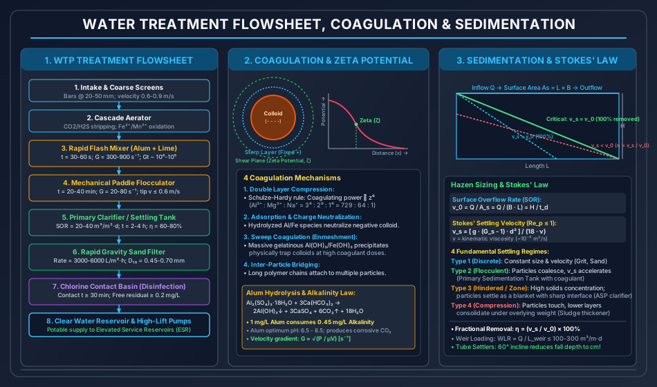
3.1 Unit Operation Sequence of Conventional Municipal WTP
Raw surface water (rivers, impounding reservoirs) carrying suspended silt, organic color, colloidal clay, and enteric pathogens is routed through the following unit processes:
- Intake & Screens: Racks of steel bars inclined at with clear openings of (approach velocity ) to intercept floating logs, branches, leaves, and debris.
- Aerator: Promotes gas-liquid interfacial mass transfer.
- Flash Mixer: Rapid, high-intensity dispersion of coagulant chemicals into the raw water stream ().
- Flocculator: Gentle, low-shear agitation () allowing micro-flocs to collide and agglomerate into large, settleable macro-flocs.
- Sedimentation Basin: Gravitational separation of settleable flocs ().
- Filtration Bed: Granular silica sand media removing residual non-settleable micro-flocs, colloidal turbidity, and pathogenic cysts.
- Disinfection Basin: Chemical destruction of pathogenic microorganisms to ensure zero viable coliforms in distribution.
3.2 Aeration Gas-Transfer Kinetics (Two-Film Theory)
Aeration exposes water to atmospheric air to strip undesirable dissolved gases and introduce oxygen.
- Key Objectives:
- Expulsion of Carbon Dioxide (): Strips aggressive carbonic acid, elevating pH and dramatically reducing the corrosivity of water toward municipal distribution mains.
- Removal of Hydrogen Sulfide (): Strips volatile , eliminating offensive "rotten-egg" odors and reducing chlorine demand.
- Oxidation of Soluble Iron and Manganese: Converts soluble, un-oxidized ferrous () and manganous () ions into insoluble gelatinous precipitates:
- Volatile Organic Compounds (VOC) Stripping: Removes algal taste-and-odor metabolites (geosmin, MIB).
- Two-Film Transfer Kinetics (Lewis & Whitman): where is dissolved gas concentration at time , is saturation concentration at the ambient temperature and partial pressure (Henry's Law ), is liquid film mass transfer coefficient, and is specific interfacial contact surface area per unit volume.
- Types of Aerators:
- Cascade Aerators: Water drops over a series of concrete steps or circular trays ( height per drop; total head ). Space-efficient, low maintenance; most widely used in India.
- Spray Aerators: Upward-directed hydraulic nozzles under pressure (), atomizing water into fine droplets (). Highly efficient, but requires high pumping energy and vulnerable to wind drift.
- Diffused Air Aerators: Compressed air bubbled through perforated diffuser tubes at the bottom of a basin ().
- Tray / Slat Aerators: Packed towers filled with coke, crushed stone, or slotted wooden slats.
4. Coagulation & Flocculation Mechanics
Natural turbidity, color, and clay particles in water range from to . Because of their minuscule mass and high specific surface area, gravitational settling velocities are negligibly slow (; a colloidal clay particle requires to settle !). Furthermore, colloidal particles carry net negative electrical surface charges that cause them to mutually repel, creating a stable, non-settling suspension.
4.1 The Electrical Double Layer & Zeta Potential
A colloidal particle in water develops a primary negative surface charge (from isomorphic substitution in clay crystal lattices, preferential adsorption of , or ionization of carboxyl/hydroxyl functional groups).
- Stern Layer: A rigid, immobilized inner monolayer of dehydrated positive counter-ions firmly bound to the particle surface by electrostatic attraction and chemical sorption.
- Gouy-Chapman Diffuse Layer: A dynamic outer zone of hydrated cations extending into the bulk solution, where electrostatic attraction balances thermal kinetic diffusion.
- Shear Plane (Plane of Slipping): The boundary separating the fluid adhering to the moving particle from the bulk liquid.
- Zeta Potential (): The electrostatic potential difference measured across the plane of shear relative to the electroneutral bulk solution: where is double layer thickness, is net charge, and is dielectric constant. In typical untreated river waters, . Inter-particle electrostatic repulsion dominates over attractive London-van der Waals forces.
4.2 Four Destabilization Mechanisms
Coagulation destabilizes the colloidal suspension via four primary physicochemical pathways:
- Compression of the Electrical Double Layer:
- Increasing the ionic strength of the water compresses the diffuse layer thickness (), allowing van der Waals attractive forces to dominate at closer contact distances.
- Schulze-Hardy Rule: The coagulating efficiency of an electrolyte is proportional to the sixth power of the counter-ion valence (): Trivalent aluminum () or ferric () ions are over more effective than monovalent sodium ().
- Adsorption and Charge Neutralization:
- Positively charged polymeric metal-hydroxy complexes (such as and ) adsorb specifically onto the negatively charged colloidal surfaces, reducing the Zeta potential toward zero (, the isoelectric point).
- Restabilization Danger: Overdosing coagulant reverses the charge to positive (), re-stabilizing the suspension.
- Sweep Coagulation (Enmeshment in Precipitate):
- At high coagulant dosages and neutral-to-alkaline pH, aluminum or ferric ions rapidly exceed their solubility limits, precipitating as massive, voluminous gelatinous metal hydroxides ( or ).
- As these sticky hydroxide precipitates settle, they physically capture, enmesh, and sweep colloidal particles down with them. Operates independently of colloidal charge.
- Inter-Particle Bridging:
- Long-chain synthetic or natural polymers (polyelectrolytes, polyacrylamides) adsorb simultaneously onto multiple colloidal particles, anchoring them together into large, settleable floc networks.
4.3 Coagulant Chemistry & Alkalinity Stoichiometry
1. Alum (Filter Alum, Aluminum Sulfate, )
- Most widely utilized commercial coagulant in municipal water treatment.
- Molar Mass of Hydrated Alum .
- Hydrolysis Reaction in the Presence of Natural Alkalinity:
- Optimum Operating pH: . (Below pH , soluble persists; above pH , soluble aluminate forms, increasing residual toxic aluminum in treated water).
- Stoichiometric Alkalinity Consumption: If raw water lacks sufficient natural bicarbonate alkalinity (), external alkalinity must be dosed in the form of Hydrated Lime (), Quicklime (), or Soda Ash ().
- By-Product Formation: Each of alum produces of free , lowering water pH and inducing corrosivity.
2. Iron Salts (Ferric Chloride, Ferrous Sulfate, Chlorinated Copperas)
- Ferric Chloride (): Rapid hydrolysis across a broad pH range (). Generates dense, heavy ferric hydroxide flocs () that settle faster than alum flocs. Corrosive liquid; requires rubber-lined storage tanks.
- Copperas (Ferrous Sulfate, ): Requires dissolved oxygen and alkaline conditions () to oxidize ; commonly dosed in conjunction with lime.
- Chlorinated Copperas: Reacting copperas with chlorine in a ratio yields a stoichiometric mixture of ferric sulfate and ferric chloride: Operates exceptionally well for removing industrial color at low pH () and manganese at high pH ().
4.4 The Jar Test Procedure
The standard laboratory method for evaluating coagulation effectiveness:
- Six beakers filled with raw water and placed beneath a multi-spindle jar test paddle apparatus.
- Dosed with incrementally increasing dosages of coagulant (e.g., ).
- Rapid Mix Phase: Flash mixed at for .
- Flocculation Phase: Slow mixed at for .
- Sedimentation Phase: Paddles stopped; flocs allowed to settle quiescently for .
- Supernatant sampled from a tap below the surface and tested for residual turbidity (NTU), color, and residual aluminum. The lowest coagulant dose yielding the target turbidity () represents the Optimum Coagulant Dose.
4.5 Rapid Flash Mixer & Mechanical Flocculator Design
Velocity Gradient Formulation (Camp & Stein, 1943)
Agitation intensity is governed by the root-mean-square Velocity Gradient ():
where:
- is total power dissipated in the fluid ().
- is dynamic viscosity of water ( at ).
- is tank volume ().
- Camp Number (): Dimensionless collision parameter. where is hydraulic detention time ().
Design Standards for Mixing Units (CPHEEO)
| Design Parameter | Rapid Flash Mixer | Mechanical Paddle Flocculator |
|---|---|---|
| Detention Time () | ||
| Velocity Gradient () | (Tapered: ) | |
| Camp Number () | ||
| Paddle / Impeller Peripheral Speed | (high-speed propeller) | (strictly to prevent floc tear) |
| Paddle Area to Basin Cross-Section Ratio | — | of vertical tank plane |
| Power Consumption () Formula |
5. Sedimentation Mechanics & Basin Sizing
5.1 The Four Settling Regimes
- Type 1 (Discrete Settling): Plain sedimentation of non-flocculent, unhindered individual particles (e.g., mineral grit, coarse sand). Particle retains constant size, shape, and settling velocity ().
- Type 2 (Flocculent Settling): Dilute suspension of coalescing particles (coagulated water in primary clarifiers). As particles settle, they collide, aggregate, grow in size, and accelerate downward.
- Type 3 (Hindered / Zone Settling): Intermediate solids concentration () where inter-particle repulsive forces create a continuous settling blanket. A sharp liquid-solid clarification interface descends as a uniform zone (secondary clarifiers in biological Activated Sludge Process).
- Type 4 (Compression Settling): High solids concentration () where particles physically touch and form a mechanical lattice; consolidation occurs solely by structural deformation under the weight of overlying layers (gravity sludge thickeners).
5.2 Mechanics of Type-1 Discrete Settling (Stokes' Law)
Consider a spherical particle of diameter and mass density settling in water of density and dynamic viscosity . Three forces act on the particle:
- Submerged Gravitational Weight:
- Hydrodynamic Drag Force:
Equating at terminal settling velocity:
where is specific gravity of particle.
Drag Coefficient Regimes
- Laminar Regime (Stokes' Flow: Particle Reynolds Number ): Substituting into the velocity equation:
- Transition Regime ():
- Turbulent Regime (Newton's Flow: ):
5.3 Hazen's Theory of Ideal Continuous-Flow Settling Basins
Hazen (1904) modeled sedimentation in an ideal rectangular basin of length , width , and water depth :
- Assumptions:
- Flow is steady, uniform, and purely horizontal across cross-section ().
- Particles entering the basin are uniformly dispersed across the vertical inlet zone.
- Any particle reaching the bottom sludge boundary layer is permanently captured and removed.
Surface Overflow Rate (SOR / Hydraulic Surface Loading)
The total fluid residence time in the basin is:
A particle entering at the extreme top water surface at the inlet will just reach the floor at the outlet if its vertical settling velocity equals:
- The Hazen Sizing Law: The clarifying capacity of a horizontal sedimentation tank is strictly independent of depth (); it depends solely on flow rate () and plan surface area ()!
- Removal Efficiency:
- Any particle having settling velocity will be 100% removed, regardless of the depth at which it enters the tank.
- Any particle having settling velocity will be partially removed, with removal fraction:
Codal Design Parameters for Sedimentation Tanks (CPHEEO)
- Plain Sedimentation (No chemicals): ; detention time .
- Coagulated Clarifiers (PST with Alum): ; detention time .
- Length-to-Width Ratio: (minimizes short-circuiting dead zones).
- Water Depth (): (provides scour buffer and sludge storage).
- Weir Loading Rate (): (Excessive weir loading creates high localized upflow velocity near effluent troughs, pulling settled flocs over the weir).
- High-Rate Tube Settlers & Lamella Plates:
- Modules of PVC or fiberglass tubes inclined at (steep enough for settled sludge to slide downward under gravity into the lower hopper).
- Tube diameter , length .
- Reduces critical settling distance from to , allowing surface overflow rates to be increased by for the same footprint!
6. Granular Media Filtration: Slow Sand vs Rapid Sand Filters
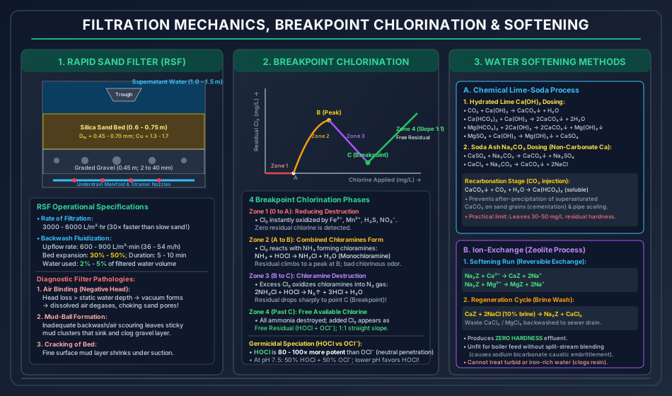
Filtration purifies water by passing it downward through a porous bed of granular silica sand, gravel, and anthracite.
6.1 Slow Sand Filters (SSF) vs Rapid Sand Gravity Filters (RSF)
The following master comparative matrix highlights the design, physical, biological, and operational distinctions:
| Design & Operational Parameter | Slow Sand Filter (SSF) | Rapid Sand Filter (Gravity RSF) |
|---|---|---|
| Rate of Filtration | () | () — faster! |
| Sand Media Effective Size () | (Fine sand) | (Coarser sand) |
| Uniformity Coefficient () | (Heterogeneous) | (Uniform, strictly rounded) |
| Depth of Sand Bed | ||
| Underlying Gravel Layer | ( graded) | ( graded in 4 layers) |
| Primary Purification Mechanism | Biological Action (Schmutzdecke skin) | Physicochemical Depth Straining & Adsorption |
| Pre-Treatment Permitted | Plain Sedimentation ONLY (Raw turbidity ) | Full Coagulation + Flocculation + Sedimentation |
| Coagulant Use | PROHIBITED (Alum flocs choke sand surface instantly) | MANDATORY (Requires micro-floc formation) |
| Cleaning Method | Surface Scraping: Top shaved off manually | Upflow Backwash: Clean water pumped upward with air scour |
| Backwash Rate & Expansion | No backwashing | ; bed expanded by |
| Water Consumed in Cleaning | of filtered water | of total filtered water |
| Filter Run Period (Cycle) | ||
| Bacterial Removal Efficiency | (2 to 3-log reduction) | (relies on post-chlorination) |
| Color Removal Efficiency | Low () | Excellent ( with alum) |
| Land Footprint Requirement | Very large (uneconomical for large cities) | Compact ( the land area of SSF) |
6.2 Biological Purification in Slow Sand Filters (Schmutzdecke)
When raw water flows through a newly packed slow sand filter, purification is initially poor. Over of continuous operation, a dark, slimy, gelatinous zoogleal biological film develops on the top of the sand bed, termed the Schmutzdecke (German for "dirty layer"):
- Consists of a living consortium of algae (Diatoms, Chlorophyceae), active bacteria, flagellates, protozoan amoebae, and rotifers.
- As water trickles past, organic matter and pathogens are captured by electrostatic interception. Predatory protozoa feed on enteric bacteria and viruses, metabolizing them into inert inorganic nitrates, sulfates, and carbon dioxide.
- Ripened slow sand filters achieve removal of Cryptosporidium oocysts and Giardia cysts without chemical dosing.
6.3 Filtration Hydraulics & Head Loss in Rapid Sand Beds
When water passes downward through a clean granular bed of porosity , depth , and specific surface area , head loss is governed by the Kozeny-Carman Equation (for laminar flow through porous media):
For non-uniform sand stratified into size fractions:
where is Kozeny constant, is kinematic viscosity, is filtration rate (), and is mass fraction of sand of geometric mean diameter .
- Clean Filter Head Loss: Typically .
- Terminal Head Loss: Over , trapped suspended matter chokes the intergranular pore voids, driving head loss up to . At this terminal threshold, the filter must be taken offline and backwashed.
6.4 Backwash Fluidization Hydraulics
During backwashing, clean treated water is pumped upward through the underdrain system. At the Minimum Fluidization Velocity (), the upward drag force equals the submerged buoyant weight of the sand grains, lifting and fluidizing the bed:
where is particle sphericity ( for sand) and .
- Bed Expansion: The fluidized bed expands to a new height : Operating standards require an expansion of () to ensure individual sand grains rub against one another, scouring off adhering mud and floc.
- Air Scouring: High-pressure air ( at ) is injected for prior to water wash to shatter sticky mud crusts.
6.5 Diagnostic Filter Operational Pathologies
- Air Binding (Negative Head Development):
- Mechanics: As solids accumulate in the upper sand layers, resistance increases. When the cumulative head loss through the top sand exceeds the static water depth overlying the bed, the pressure inside the lower sand layer drops below atmospheric pressure, creating a localized vacuum (Negative Head).
- Consequence: Dissolved air spontaneously degases from the water, forming microscopic air bubbles that become trapped in pore throats. The filter bed becomes air-bound, choking flow completely and blowing craters during backwash.
- Mud-Ball Formation:
- Mechanics: Inadequate backwash velocity or insufficient air scouring allows clay and alum floc to coalesce into sticky, dense, round balls ().
- Consequence: Mud-balls grow heavier, sink through fluidized sand, and settle onto the gravel foundation, causing severe flow maldistribution and gravel displacement. Remedied by surface wash jets () or manual caustic soda soaking.
- Cracking of the Filter Bed:
- Mechanics: Fine mud adhering to the top sand contracts under negative head suction, tearing the surface layer into jagged shrinkage cracks ( wide). Turbid water short-circuits directly through cracks into the effluent without filtration.
- Sand Boiling (Gravel Displacement):
- Caused by sudden surges in backwash pumping or defective strainer nozzles, creating high-velocity upward jets that blow gravel out of position, allowing fine filter sand to leak into the underdrain manifold.
7. Disinfection Kinetics & Breakpoint Chlorination Dynamics
Filtration removes of bacteria, but cannot guarantee zero pathogens. Disinfection destroys remaining disease-causing organisms.
7.1 Chemistry of Aqueous Chlorine
When chlorine gas () is dissolved in water, it rapidly hydrolyzes ():
Hypochlorous acid () dissociates reversibly into hypochlorite ion ():
- The HOCl vs OCl Germicidal Disparity:
- Hypochlorous Acid () is an uncharged, neutral molecule with a small molecular radius. It easily penetrates the negatively charged lipid bilayer membrane of bacterial cells, oxidizing essential respiratory enzymes and denaturing DNA.
- Hypochlorite Ion () carries a negative charge and is electrostatically repelled by bacterial cell walls.
- is more effective as a bactericide and more effective as a virucide than !
- pH Dependence: At pH , exists as active ; at pH , ; at pH , exists as sluggish . Chlorination is vastly superior at lower pH.
7.2 Formation of Chloramines (Combined Chlorine)
When water contains free dissolved ammonia ( / ), reacts in competing sequential steps:
- Chloramines represent Combined Available Residual Chlorine.
- They are weaker disinfectants than free chlorine (requiring longer contact time), but are chemically stable, persistent in long pipe networks, and do not synthesize carcinogenic trihalomethanes.
7.3 The Breakpoint Chlorination Phenomenon
When incrementally increasing doses of chlorine are added to ammonia-bearing water, residual chlorine follows a characteristic 4-zone curve:
- Zone 1 (Immediate Reducing Demand):
- Chlorine is completely reduced to inactive chloride () by inorganic reducing compounds (). Zero residual chlorine appears.
- Zone 2 (Chloramine Synthesis):
- Chlorine reacts with ammonia to form monochloramines and dichloramines.
- Measured residual chlorine rises linearly to reach a distinct peak at Point B. Water develops a strong, pungent, medicinal chlorinous odor.
- Zone 3 (Destruction of Chloramines / The Breakpoint):
- As additional chlorine is dosed past Point B, the excess chlorine oxidizes the previously formed chloramines into inert, odorless nitrogen gas () and nitrous oxide ():
- The residual chlorine concentration plummets sharply, reaching an absolute minimum at Point C — The Breakpoint.
- At the breakpoint, all ammonia is completely oxidized, and bad chlorinous tastes and odors vanish!
- Zone 4 (Free Available Residual Chlorine):
- Any chlorine added beyond Point C does not react further; it appears directly as Free Available Residual Chlorine ().
- The curve rises straight upward at a constant () slope.
- Codal Standard: Municipal chlorination must be operated strictly in Zone 4 (past the breakpoint) to guarantee a minimum free residual chlorine of after contact time in the clear water tank (and at consumer taps).
7.4 Disinfection Kinetics: Chick's Law & Chick-Watson Law
- Chick's Law (1908): Inactivation of microorganisms follows pseudo-first-order reaction kinetics: where is initial pathogen count, is survivors at time , and is reaction rate constant.
- Chick-Watson Law (1908): The rate constant depends on disinfectant concentration :
Integrating:
For a fixed target log-inactivation (e.g., , ):
where is disinfectant concentration (), is contact time (), and is coefficient of dilution ( for free chlorine).
- The product () is the universal design metric:
- E. coli 3-log kill: .
- Giardia cyst 3-log kill: .
- Cryptosporidium oocyst 3-log kill: (chlorine cannot kill Cryptosporidium; requires UV or Ozone!).
- The product () is the universal design metric:
7.5 Disinfection By-Products (DBPs) & Alternative Disinfectants
- Trihalomethanes (THMs): Free chlorine reacts with natural organic precursors (humic/fulvic acids) to produce carcinogenic organochlorines: Chloroform (), Bromoform, Chlorodibromomethane. Regulated under strict limits ().
- Alternative Disinfectants:
- Ozone (): Extremely powerful oxidant (); destroys Cryptosporidium rapidly; synthesizes zero THMs. Leaves no residual in distribution; must be supplemented with a secondary chloramine dose. High capital cost.
- Chlorine Dioxide (): Does not react with ammonia; does not form THMs; highly effective over wide pH range (). Generates chlorite and chlorate by-products.
- Ultraviolet (UV) Radiation: Mercury vapor lamps emit germicidal radiation at , dimerizing adjacent thymine bases in microbial DNA to prevent replication. Purely physical; no chemicals, no DBPs, no residual.
8. Water Softening Technologies
Water with Total Hardness requires softening for municipal and industrial use.
8.1 The Chemical Lime-Soda Process
Hardness is removed by chemical precipitation as insoluble Calcium Carbonate (, ) and Magnesium Hydroxide (, ).
Stoichiometric Chemical Reactions
- Neutralization of Free Dissolved Carbon Dioxide (consumes lime):
- Precipitation of Calcium Carbonate Hardness (consumes lime):
- Precipitation of Magnesium Carbonate Hardness (consumes double lime):
- Precipitation of Non-Carbonate Magnesium Hardness (consumes lime + soda): (Note: Replaces with an equivalent amount of , creating non-carbonate calcium hardness).
- Precipitation of Non-Carbonate Calcium Hardness (consumes soda ash):
Recarbonation
Precipitation reactions leave treated water supersaturated with fine, colloidal (). If unfiltered, this crystallizes onto rapid sand grains (cementing them into rock) and incrusts distribution pipes. Water is recarbonated by bubbling carbon dioxide gas ():
- Practical Limit: The lime-soda process cannot produce zero hardness due to residual solubility; practical effluent contains residual hardness as .
8.2 Zeolite / Synthetic Cation Exchange Process
- Chemistry: Water passes through a column of synthetic ion-exchange resin (sulfonated polystyrene beads) or natural greensand zeolite containing exchangeable sodium ions ():
- Characteristics:
- Produces Zero Hardness Water ().
- Replaces all hardness cations with sodium ions on a strict equivalent-for-equivalent basis ( yields ).
- Unfit for high-pressure boiler feed without blending (causes sodium bicarbonate decomposition and caustic embrittlement).
- Regeneration Cycle: When resin capacity is exhausted, the unit is taken offline, backwashed, and regenerated by soaking with a concentrated Sodium Chloride brine solution (): Waste calcium and magnesium chloride brine is flushed to drain.
9. Step-by-Step Analytical Derivations & Quantitative Formulations
9.1 Mathematical Derivation of Stokes' Terminal Settling Velocity
Consider an isolated spherical particle of diameter , density , settling under gravity in an infinite, quiescent Newtonian fluid of density and dynamic viscosity .
- Downward Gravitational Force:
- Upward Buoyant Force (Archimedes' Principle):
- Net Submerged Downward Driving Force:
- Upward Hydrodynamic Viscous Drag Force: From dimensional analysis:
- Equilibrium at Terminal Velocity (): Canceling common terms:
- Substituting Laminar Drag Coefficient (): Squaring both sides:
9.2 Derivation of Fractional Particle Removal in Hazen Settling Basin
In an ideal rectangular horizontal settling basin of length , depth , and width :
- Horizontal flow velocity:
- A particle having settling velocity enters the basin at elevation above the basin floor ().
- The time required for this particle to settle to the floor is:
- The maximum horizontal residence time available is:
- The particle is successfully captured if:
- Assuming particles are uniformly distributed across the entire vertical inlet plane (height to ), the fraction of particles entering at or below height that will be removed is:
10. Solved Numerical Examples (Pre-Calculated & Python-Verified)
Problem 1: Coagulation Alkalinity Stoichiometry & Flash Mixer Design
A municipal water treatment plant is designed to treat () of surface water. Laboratory jar testing establishes an optimum alum dosage of of commercial hydrated alum , which has a molar mass of . The raw river water has an initial natural bicarbonate alkalinity of .
Calculate:
- The total quantity of alum consumed daily, in metric tonnes per day.
- The total alkalinity consumed by the alum reaction, in .
- The alkalinity deficit, and the daily requirement (in ) of commercial quicklime ( of purity) needed to maintain a minimum residual buffering alkalinity of in the coagulated water.
- The required dimensions and motor power () for a square rapid flash mixing tank operating with a detention time and a velocity gradient at ().
Solution:
Step 1: Daily Alum Requirement:
Step 2: Alkalinity Consumed by Alum: Stoichiometric reaction:
Step 3: Alkalinity Deficit & Commercial Lime Sizing:
- Total alkalinity required:
- Natural raw water alkalinity .
- Alkalinity Deficit:
- Equivalent Pure Quicklime ():
- Adjusting for purity:
- Daily Commercial Lime Consumed:
Step 4: Rapid Flash Mixer Design:
- Volumetric flow rate:
- Basin Volume:
- Assuming square tank with depth ():
- Dissipated Fluid Power ():
Problem 2: Sedimentation Basin Design & Particle Settling Efficiency
A rectangular horizontal-flow primary settling basin is designed to treat () of coagulated municipal water. Design criteria:
- Surface Overflow Rate:
- Detention Time:
- Basin Geometry: Length-to-Width Ratio
- Water Properties: Density , kinematic viscosity ,
- Silt/Sand Particle Specific Gravity:
Determine:
- Basin plan dimensions (Length , Width ) and effective water depth ().
- Overflow rate expressed in .
- The minimum diameter () of spherical discrete particles that will be completely removed by this basin, and verify laminar Stokes flow ().
- The fractional removal efficiency () of fine particles with diameter ().
Solution:
Step 1: Basin Geometry & Plan Area:
- Plan surface area:
- Width and Length ():
- Total Basin Volume ():
- Effective Water Depth ():
Step 2: Overflow Rate in mm/s:
Step 3: Minimum Particle Diameter for 100% Removal: For removal, . Using Stokes' Law:
Check Particle Reynolds Number:
Stokes' laminar settling regime holds valid.
Step 4: Fractional Removal Efficiency for ():
Problem 3: Rapid Sand Filter Bed Sizing & Bleaching Powder Disinfection
A rapid sand gravity filter plant is to treat of coagulated, settled water. Operational design specifications:
- Daily filter operating cycle: total ( filtration, offline for backwashing and drainage).
- Design filtration rate: ().
- The plant is divided into equal rectangular filter beds with a length-to-width ratio .
- Backwash water is pumped upward at a rate of for per bed per day.
- Chlorination: Laboratory chlorine demand tests indicate a demand of . To ensure adequate safety, a free residual chlorine of is required after contact time. Commercial bleaching powder with available chlorine is used.
Calculate:
- Total sand surface area required and the dimensions (Length and Width ) of each of the 4 filter units.
- Volume of backwash water consumed per bed per wash (), total daily backwash water (), and the percentage of treated water consumed in backwashing.
- Total chlorine dosage (), daily pure chlorine demand (), and daily commercial bleaching powder required ().
Solution:
Step 1: Filter Bed Surface Area & Dimensions:
- Net volume to be filtered per hour during active filtration:
- Total surface area required:
- Area per bed ():
- Bed Dimensions ():
Step 2: Backwash Water Requirements:
- Backwash rate:
- Volume per bed per wash ():
- Total daily backwash water for all 4 beds:
- Percentage of treated water consumed in backwashing: (Fully compliant with the CPHEEO statutory limit of ).
Step 3: Chlorination & Bleaching Powder Sizing:
- Total design chlorine dosage:
- Daily Pure Chlorine Consumed:
- Commercial Bleaching Powder ( available chlorine):
11. Common Misconceptions, Pitfalls & Exam Traps
[!WARNING] Trap 1: Hazen Settling Area Independence from Depth: A classic GATE/ESE question asks: "If the depth of a settling basin is doubled while keeping flow and plan area constant, what happens to settling efficiency?" Answer: The settling efficiency remains completely unchanged! Efficiency depends strictly on . While depth doubles detention time , it also doubles the distance the particle must fall (). Depth affects only horizontal velocity and scouring protection.
[!CAUTION] Trap 2: Alum in Slow Sand Filters: Coagulants like alum or ferric chloride MUST NEVER be applied to slow sand filters! Gelatinous alum flocs cannot penetrate sand pores and immediately form an impermeable cake on the bed surface, blinding the filter within hours. Slow sand filters rely purely on natural biological Schmutzdecke maturation.
[!IMPORTANT] Trap 3: Negative Head vs Vacuum in Filtration: Negative head does NOT mean backflow or reverse water direction. It denotes a condition where static head loss through the clogged top sand layer exceeds the hydrostatic head of water overlying the sand, causing absolute pore pressure to drop below local atmospheric pressure. This pulls dissolved air out of solution, causing Air Binding.
[!WARNING] Trap 4: Breakpoint Minimum vs Free Chlorine: At the Breakpoint (Point C), residual chlorine is at a local minimum, NOT a maximum. Odors vanish at Point C because chloramines are fully destroyed. Free available residual chlorine appears strictly beyond Point C (Zone 4).
[!NOTE] Trap 5: Lime-Soda Softening Effluent Hardness: The Lime-Soda process cannot achieve zero hardness due to the slight inherent solubility of () and (). Practical effluent contains . Only the Zeolite Cation Exchange process produces true zero hardness.
12. Practice Problems (Curated for Competitive Examinations)
Level 1: Objective & Conceptual (SSC JE / RRB JE / State AE)
-
The biological active layer formed on the surface of a slow sand filter responsible for pathogen destruction is called:
- (A) Floc blanket
- (B) Schmutzdecke
- (C) Sludge carpet
- (D) Bio-film filter media Answer: (B) Schmutzdecke (dirty layer).
-
According to the Schulze-Hardy rule, the coagulating power of trivalent aluminum () compared to monovalent sodium () is approximately:
- (A)
- (B)
- (C)
- (D) Answer: (D) .
-
In water treatment, air binding in rapid sand filters is primarily caused by:
- (A) Excessive backwash pump pressure
- (B) Development of negative head exceeding static water depth, causing dissolved air release
- (C) Growth of filamentous algae in sand pores
- (D) Excessive coagulant dosing Answer: (B) Negative head development leads to dissolved air release.
-
The chemical species of chlorine that possesses the most potent bactericidal disinfection efficiency is:
- (A) Hypochlorite ion ()
- (B) Hypochlorous acid ()
- (C) Monochloramine ()
- (D) Chloride ion () Answer: (B) ( more potent than ).
-
In the chemical lime-soda softening process, recarbonation with is performed to:
- (A) Destroy pathogenic coliforms
- (B) Convert supersaturated into soluble to prevent pipe incrustation
- (C) Strip hydrogen sulfide gas
- (D) Precipitate non-carbonate sulfate hardness Answer: (B) Converts supersaturated to soluble .
Level 2: Analytical & Multi-Step (GATE CE / UPSC ESE)
-
A continuous-flow settling tank of depth and length operates with a horizontal velocity of . What is the minimum settling velocity of particles in that will be removed by this tank?
- (A)
- (B)
- (C)
- (D) Answer: (B)
- Detention time: .
- Critical settling velocity: .
-
A rapid sand filter is backwashed at a rate of . If the initial unexpanded sand depth is with porosity , and the porosity of the fluidized expanded sand bed is , what is the expanded depth of the sand bed?
- (A)
- (B)
- (C)
- (D) Answer: (C)
- Solid volume conservation: .
- ( expansion).
-
A water treatment plant doses of alum to treat river water. If the natural bicarbonate alkalinity is , how much additional alkalinity as must be supplied to ensure a residual alkalinity of ?
- (A)
- (B)
- (C)
- (D) Answer: (C)
- Alkalinity consumed .
- Total required .
- Deficit to add .
13. Quick Revision Summary & Memory Hooks
Core Numerical Rules & Design Constants
- WTP Unit Process Order: Intake Aeration Rapid Mix (Alum) Flocculator Clarifier Rapid Filter Disinfection Clear Water Tank.
- Alum Consumption Rule: consumes and generates (Optimum pH ).
- Velocity Gradient (): . Flash mix: (). Flocculator: ().
- Stokes' Settling Velocity: ().
- Hazen Overflow Sizing: . 100% removal if ; fractional . Clarifying capacity is independent of depth!
- Slow Sand vs Rapid Sand Filters:
- Filtration Rate: SSF vs RSF ().
- Effective Size : SSF vs RSF .
- Cleaning: SSF = Scraping Schmutzdecke vs RSF = High-rate backwash ( expansion).
- Backwash Water: RSF consumes of treated water.
- Breakpoint Chlorination: Zone 1 (Reducing demand) Zone 2 (Chloramines peak) Zone 3 (Chloramines destroyed down to Point C Breakpoint) Zone 4 (Free available chlorine , slope 1:1).
- Potency: is more germicidal than (neutral penetration favored at lower pH).
- Chick-Watson Law: .
- Softening: Lime precipitates carbonate hardness & ; Soda ash precipitates non-carbonate calcium; Zeolite yields true zero hardness.