Soil Permeability, Darcy's Law, Laboratory & Field Permeameters, Stratified Soils & 2D Seepage Flow Nets
In this chapter (8 topics)
On this page
- 1. Module Overview & Learning Objectives
- Core Exam Focus Areas
- 2. Fundamental Principles & Physics of Soil Permeability
- 2.1 Darcy's Law (Henri Darcy, 1856)
- 2.2 Limits of Validity of Darcy's Law
- 3. Mathematical Derivations & Analytical Formulations
- 3.1 Discharge Velocity vs. True Seepage Velocity
- 3.2 Analytical Derivation of Kozeny-Carman Equation
- 3.3 Physical Factors Governing Soil Permeability
- 3.4 Allen Hazen's Empirical Formulation
- 4. Visual Master Diagram: Darcy's Law & Laboratory Permeameters
- 5. Laboratory Determination of Permeability (IS 2720 Part 17)
- 5.1 Constant Head Permeameter (For Coarse Granular Soils, k > 10-3 cm/s)
- 5.2 Falling Head (Variable Head) Permeameter (For Fine Soils, k < 10-3 cm/s)
- 6. Visual Master Diagram: Stratified Soil Permeability & 2D Seepage Flow Nets
- 7. Equivalent Permeability of Stratified Soil Deposits
- 7.1 Flow Parallel to Bedding Planes (Horizontal Flow, kx)
- 7.2 Flow Perpendicular to Bedding Planes (Vertical Flow, kz)
- 7.3 Fundamental Anisotropy Theorem
- 8. Two-Dimensional Seepage Theory & Flow Nets
- 8.1 Derivation of 2D Laplace's Equation
- 8.2 Flow Net Geometry & Constitutive Rules
- 8.3 Seepage Calculations from Flow Nets
- 9. Solved Numerical Problems (Step-by-Step, Pre-Calculated)
- Problem 1: Constant Head vs. Falling Head Permeameter (GATE CE / UPSC ESE)
- Problem 2: Equivalent Permeability of Stratified Subsoil (GATE CE / SSC JE)
- Problem 3: Flow Net Seepage, Uplift & Exit Gradient Analysis (UPSC ESE / GATE CE)
- 10. Comparative Engineering Analysis & Multi-Exam Question Patterns
- 11. Common Misconceptions, Pitfalls & Pro-Tips
- Critical Traps to Avoid in Competitive Exams
- 12. Key Reference Formulas & Summary Table
1. Module Overview & Learning Objectives
Permeability (or hydraulic conductivity, ) is defined as the ease with which a fluid (typically pore water) flows through the interconnected void spaces of a porous soil medium under a hydraulic gradient. It is one of the most consequential parameters in geotechnical engineering, governing:
- Rate of settlement of structures founded on compressible saturated fine-grained soils (1D consolidation).
- Seepage discharge and leakage rates beneath concrete dams, through earthen embankments, and into cofferdams.
- Stability of slopes, cuts, and retaining walls against hydrodynamic seepage forces.
- Liquefaction, piping, and quicksand failure at the downstream exit face of hydraulic structures.
- Design of subsurface dewatering systems, filter drains, and landfill containment clay liners.
+----------------------------------------------------------------------------------------------------+
|                                    PERMEABILITY SPECTRUM ACROSS SOILS                              |
+----------------------+----------------------+----------------------+-------------------------------+
| SOIL TYPE            | k (cm/s)             | DRAINAGE CAPACITY    | LABORATORY / FIELD TEST       |
+----------------------+----------------------+----------------------+-------------------------------+
| Clean Gravels        | > 1.0                | Exceptionally Rapid  | Constant Head / Pumping Test  |
| Clean Sands, Sand-Gravel | 1.0 to 10^-3     | Good / Free Draining | Constant Head Permeameter     |
| Fine Sands, Silts    | 10^-3 to 10^-7       | Poor / Slow          | Falling Head Permeameter      |
| Intact Clays         | < 10^-7 (to 10^-10)  | Practically Impervious| Falling Head / Oedometer Consol|
+----------------------+----------------------+----------------------+-------------------------------+
Core Exam Focus Areas
- GATE CE: Derivation of discharge velocity () vs. seepage velocity (); Kozeny-Carman relation (, ); Falling head permeameter time and head calculations; Stratified soil parallel () vs. perpendicular () equivalent permeability; 2D Laplace seepage equation; Flow net shape factor (), seepage calculation (), and exit gradient ().
- UPSC ESE: Detailed derivation of constant head and variable head permeameter equations; Derivation of weighted arithmetic mean for horizontal flow and weighted harmonic mean for vertical flow; Anisotropic soil transformation (, ); Uplift pressure distribution under dam foundations.
- SSC JE / State AE / RRB JE: Darcy's law validity condition (); Hazen's empirical rule (); Constant head test for coarse soils vs. falling head for fine soils; Intermediate head relation ( for equal time intervals); Factor of safety against piping ().
2. Fundamental Principles & Physics of Soil Permeability
2.1 Darcy's Law (Henri Darcy, 1856)
Through experimental investigations on the flow of water through sand filter columns, Henri Darcy established that for laminar flow through saturated granular soils, the rate of flow (discharge ) is directly proportional to the cross-sectional area of the soil bed () and the hydraulic gradient ():
Where:
- is the volumetric discharge rate ( or ).
- is the coefficient of permeability or hydraulic conductivity ( or ). It has dimensions of velocity ().
- is the dimensionless hydraulic gradient, defined as the loss of hydraulic head () per unit length of seepage path ():
- is the total gross cross-sectional area of the soil mass perpendicular to the direction of flow ( or ).
2.2 Limits of Validity of Darcy's Law
Darcy's law is valid only for laminar flow where viscous shearing forces dominate over inertial forces. Flow regime in porous media is governed by Reynolds number:
Where is the discharge velocity, is water density, is dynamic viscosity, and is the representative pore size or grain diameter ( or ).
- Laminar Flow Regime: Darcy's law holds strictly when .
- In typical natural soils (sands, silts, clays), is well below , ensuring universal validity.
- In very coarse, open-graded gravels, rockfills, or under massive hydraulic gradients near well screens, turbulent flow develops ( to ), where with (typically ).
3. Mathematical Derivations & Analytical Formulations
3.1 Discharge Velocity vs. True Seepage Velocity
Darcy's discharge velocity () is a superficial, fictitious velocity based on the entire macroscopic cross-sectional area (which includes both soil solid grains and empty pores):
However, water cannot physically penetrate through solid mineral grains; it can only flow through the tortuous interconnected void channels whose actual flow area is . By the principle of mass continuity:
Where is the true seepage velocity (average interstitial linear velocity of fluid particles):
Multiplying numerator and denominator by length :
Where is the porosity (). Therefore:
Expressing porosity in terms of void ratio ():
Critical Consequence: Since porosity (typically ):
In contaminant transport, tracer migration, and seepage erosion, the actual velocity of particle movement is governed by , never by .
3.2 Analytical Derivation of Kozeny-Carman Equation
Modeling the interconnected void network as an array of parallel tortuous capillary tubes, Poiseuille's law gives the average laminar flow velocity in a capillary tube of radius :
The hydraulic radius of the void channels is defined as:
Where is the specific surface area per unit volume of solid particles (). Substituting into Poiseuille's formulation and integrating over the porous continuum yields the classical Kozeny-Carman equation:
Where:
- is a pore shape factor ().
- is the tortuosity ().
- is a composite dimensionless pore geometry factor.
- is dynamic fluid viscosity ( or ).
- is unit weight of water ().
- is the effective particle diameter.
3.3 Physical Factors Governing Soil Permeability
From the Kozeny-Carman equation, the governing dependencies are explicitly identified:
- Grain Size (): . Permeability is overwhelmingly dictated by the smallest fraction. Coarse soils have orders-of-magnitude larger pores than fine clays.
- Void Ratio (): . As soil is compacted and decreases, permeability plummets non-linearly. A semi-log plot of vs. is approximately linear.
- Fluid Viscosity and Temperature (): . Fluid viscosity decreases with increasing temperature (). To standardize laboratory measurements, measured at test temperature is normalized to :
- Degree of Saturation (): Entrapped air bubbles block void channels, dramatically restricting flow. Saturated permeability () is to times higher than partially saturated permeability.
- Soil Fabric / Structure: At identical void ratio, a flocculated fabric has 10 to 100 times higher permeability than a dispersed fabric.
3.4 Allen Hazen's Empirical Formulation
For uniform, clean filter sands (, ), Allen Hazen established:
Where:
- is in .
- is the effective grain size in .
- is Hazen's empirical constant, typically ranging between and (standard default ).
4. Visual Master Diagram: Darcy's Law & Laboratory Permeameters
The following architectural diagram illustrates Darcy's law flow mechanics, the distinction between discharge and seepage velocities, and the experimental setups and governing mathematical derivations for both Constant Head and Falling Head permeameters.

5. Laboratory Determination of Permeability (IS 2720 Part 17)
5.1 Constant Head Permeameter (For Coarse Granular Soils, )
In coarse soils (clean sands and gravels), water flows readily, permitting the collection of measurable discharge volumes under a constant hydraulic head without requiring excessively long test durations.
Derivation of Governing Equation:
From Darcy's law:
Solving directly for :
Where:
- = total volume of water collected in measuring flask ().
- = length of soil specimen between piezometers ().
- = cross-sectional area of soil specimen mold ().
- = constant hydraulic head difference between piezometers ().
- = elapsed time duration of collection ().
5.2 Falling Head (Variable Head) Permeameter (For Fine Soils, )
In fine sands, silts, and clays, permeability is too low for the constant head method (discharge is imperceptibly small, and evaporation introduces massive error). A slender vertical standpipe of small cross-sectional area is attached to the specimen.
Derivation of Governing Differential Equation:
Let:
- = cross-sectional area of the slender standpipe.
- = cross-sectional area of the soil specimen.
- = length of the soil specimen.
- = hydraulic head at any elapsed time .
In an infinitesimal time interval , the water level in the standpipe drops by (negative rate: ). The volumetric rate of water leaving the standpipe is:
By Darcy's law, the rate of water percolating through the soil specimen at head is:
Equating inflow and outflow by mass continuity:
Separating variables:
Integrating between initial limits and final limits :
Solving explicitly for :
Equal Time Intervals Property (High-Yield Golden Rule):
If the head drops from to in time interval , and subsequently drops from to in the exact same time interval :
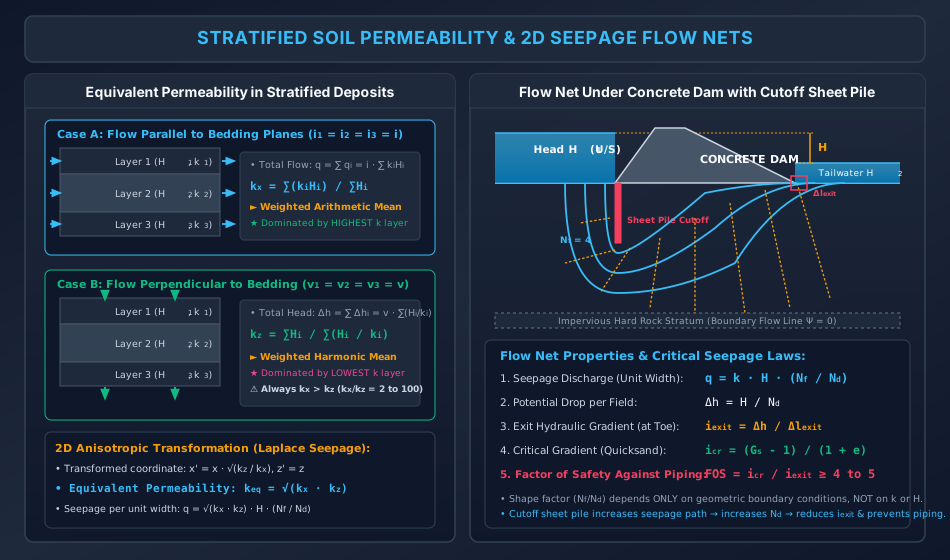
6. Visual Master Diagram: Stratified Soil Permeability & 2D Seepage Flow Nets
The following architectural diagram illustrates the analytical derivations for equivalent horizontal and vertical permeability in layered soil deposits, 2D anisotropic coordinate transformation, and the geometry and physical laws of Flow Nets beneath hydraulic structures.
7. Equivalent Permeability of Stratified Soil Deposits
Natural sedimentary soil strata are deposited in horizontal layers possessing distinct thicknesses and individual permeability coefficients .
7.1 Flow Parallel to Bedding Planes (Horizontal Flow, )
When seepage occurs parallel to the bedding planes:
- The hydraulic gradient across each layer is identical:
- The total discharge through the entire stratum of total thickness (unit width) is the sum of discharges through the individual layers:
Dividing both sides by :
Key Analytical Takeaway: is the weighted arithmetic mean of the individual layer permeabilities. It is overwhelmingly governed by the most permeable (highest ) layer. Even a thin layer of clean sand or gravel within thick clay deposits dominates .
7.2 Flow Perpendicular to Bedding Planes (Vertical Flow, )
When seepage occurs perpendicular to the bedding planes:
- By mass continuity, the flow velocity through each layer must be identical:
- The total hydraulic head loss across the entire stratum is the sum of head losses across the individual layers:
- Since :
Dividing both sides by :
Key Analytical Takeaway: is the weighted harmonic mean of the individual layer permeabilities. It is overwhelmingly governed by the least permeable (lowest ) layer. A single thin seam of impervious clay within permeable sand acts as a severe hydraulic choke, throttling vertical seepage.
7.3 Fundamental Anisotropy Theorem
For any stratified non-homogeneous soil deposit:
In natural alluvial deposits, the ratio of horizontal to vertical permeability typically ranges from to , and can exceed in varved clays.
8. Two-Dimensional Seepage Theory & Flow Nets
8.1 Derivation of 2D Laplace's Equation
Consider steady 2D seepage through an element of saturated soil of dimensions :
- Mass inflow:
- Mass outflow:
For an incompressible fluid and undeformable soil skeleton, continuity requires:
Applying Darcy's law with directional permeabilities and :
Substituting into the continuity equation:
Case 1: Isotropic Soil ()
The governing equation reduces to the classical Laplace equation:
Case 2: Anisotropic Soil ()
Dividing by :
Introducing the transformed spatial coordinate:
The equation transforms back to the standard Laplace form in the coordinate system:
The equivalent isotropic permeability of the transformed section is:
8.2 Flow Net Geometry & Constitutive Rules
A Flow Net is a graphical solution of Laplace's equation consisting of two orthogonal families of curves:
- Flow Lines (): Streamlines depicting the average trajectory of percolating water particles. No flow can cross a flow line.
- Equipotential Lines (): Contours connecting points of equal total hydraulic head . Piezometers inserted anywhere along an equipotential line will register identical water levels.
Orthogonality and Elementary Curvilinear Squares:
- Flow lines and equipotential lines intersect strictly at right angles ().
- In an isotropic flow net, the grid elements are drawn as curvilinear squares where average width equals average length :
8.3 Seepage Calculations from Flow Nets
1. Seepage Discharge per Unit Width ()
Consider a single flow channel between two adjacent flow lines:
For curvilinear squares ():
If the total net head difference across the structure is , and there are equal potential drops:
If the flow net consists of flow channels, the total seepage discharge per unit length of the hydraulic structure is:
Where:
- is called the Shape Factor of the flow net.
Invariance Theorem: The shape factor depends solely on the geometric boundary conditions of the hydraulic structure and foundation strata. It is entirely independent of the permeability , the total head , or the fluid viscosity.
2. Uplift Pressure Under Dam Foundations
At any point along the base of a concrete dam located after equipotential drops:
Taking the base of the dam as datum (), the pressure head is:
The total uplift force is obtained by integrating along the base width.
3. Exit Hydraulic Gradient & Piping Safety
Piping failure initiates at the downstream ground surface adjacent to the dam toe where upward seepage forces are most intense. The exit hydraulic gradient in the final downstream field is:
Where is the length of the downstream exit field.
The critical hydraulic gradient causing quicksand (boiling) is:
The factor of safety against piping failure is:
9. Solved Numerical Problems (Step-by-Step, Pre-Calculated)
Problem 1: Constant Head vs. Falling Head Permeameter (GATE CE / UPSC ESE)
A laboratory permeameter mold of internal diameter and length was used for two separate soil testing programs:
- Test A (Constant Head): A coarse sand specimen with porosity was tested under a constant head difference of . In an elapsed time of , exactly of water was collected in a graduated flask. Compute:
- The coefficient of permeability in and .
- The discharge velocity and the actual seepage velocity .
- Test B (Falling Head): A fine silt specimen was tested in the same mold using a standpipe of internal diameter . The hydraulic head dropped from to in . Compute:
- The coefficient of permeability in .
- The additional time required for the head to drop from to .
Solution:
Part A: Constant Head Test on Coarse Sand
-
Specimen geometric properties:
-
Coefficient of permeability ():
-
Discharge velocity ():
(Verification: )
-
Seepage velocity ():
Notice .
Part B: Falling Head Test on Fine Silt
-
Standpipe area:
-
Coefficient of permeability ():
-
Additional time for head to drop from to :
Problem 2: Equivalent Permeability of Stratified Subsoil (GATE CE / SSC JE)
A natural stratified subsoil deposit consists of three horizontal layers over an impervious bedrock:
- Layer 1 (Top): Thickness ,
- Layer 2 (Middle): Thickness ,
- Layer 3 (Bottom): Thickness ,
Compute:
- The equivalent horizontal permeability () parallel to bedding planes.
- The equivalent vertical permeability () perpendicular to bedding planes.
- The anisotropy ratio ().
- The equivalent isotropic permeability () for 2D seepage analysis.
Solution:
Total thickness:
Step 1: Horizontal Permeability () - Weighted Arithmetic Mean
(Notice: Layer 3 with contributes of the total horizontal conductance!)
Step 2: Vertical Permeability () - Weighted Harmonic Mean
(Notice: Layer 2 with accounts for of the total vertical resistance!)
Step 3: Anisotropy Ratio
Step 4: Equivalent Isotropic Permeability
Problem 3: Flow Net Seepage, Uplift & Exit Gradient Analysis (UPSC ESE / GATE CE)
A concrete gravity dam of crest length retains water with an upstream depth of and a downstream tailwater depth of . The foundation soil is a uniform fine sand with , void ratio , and coefficient of permeability . A flownet constructed for the foundation reveals:
- Number of flow channels:
- Number of equipotential drops:
- Length of the last downstream exit field adjacent to the toe:
Determine:
- The total net head causing seepage, and the head loss per potential drop .
- The seepage discharge per unit width (), and the total volumetric seepage rate () beneath the dam in and .
- The exit hydraulic gradient () at the toe.
- The critical hydraulic gradient () and the factor of safety against piping failure.
Solution:
Step 1: Net Hydraulic Head & Potential Drop
Step 2: Seepage Discharge
-
Per unit width:
-
Total seepage for entire dam length ():
Step 3: Exit Hydraulic Gradient ()
Step 4: Critical Hydraulic Gradient & Piping Factor of Safety
Engineering Assessment: A Factor of Safety of is dangerously inadequate for dam safety (standard code requirements demand ). To avert catastrophic retrogressive piping failure, an engineer must either:
- Drive a deeper vertical cutoff sheet pile wall at the upstream heel or downstream toe to increase (lengthening the flow path).
- Construct an inverted graded protective filter blanket at the downstream toe with a heavy rock toe surcharge.
10. Comparative Engineering Analysis & Multi-Exam Question Patterns
+------------------------------------+-------------------------------------------------------------------------------------------------------------------+
| EXAM LEVEL | HIGHEST YIELD TOPICS & TYPICAL QUESTION PATTERNS |
+------------------------------------+-------------------------------------------------------------------------------------------------------------------+
| GATE CE | - Numerical computation of $k_x$, $k_z$, and anisotropy ratio $k_x / k_z$ in multi-layered strata. |
| | - Variable head permeameter time calculations with geometric progression of heads ($h_2 = \sqrt{h_1 h_3}$). |
| | - Flow net shape factor $N_f / N_d$, seepage calculation, and exit gradient vs critical gradient. |
| | - Kozeny-Carman void ratio dependency ($k_1 / k_2 = [e_1^3 / (1 + e_1)] / [e_2^3 / (1 + e_2)]$). |
+------------------------------------+-------------------------------------------------------------------------------------------------------------------+
| UPSC ESE | - Complete analytical derivation of $k_x = \sum k_i H_i / \sum H_i$ and $k_z = \sum H_i / \sum (H_i / k_i)$. |
| | - Derivation of Laplace equation from 2D continuity and Darcy's law. |
| | - Anisotropic transformation $x' = x \sqrt{k_z / k_x}$ and equivalent isotropic permeability $k_{\text{eq}}$. |
| | - Detailed design and criteria for inverted protective filters (Terzaghi criteria: $D_{15F}/D_{85B} < 4 - 5$). |
+------------------------------------+-------------------------------------------------------------------------------------------------------------------+
| SSC JE / RRB JE | - Permeability test matching: Constant Head → Coarse Sand/Gravel; Falling Head → Fine Sand/Silt/Clay. |
| | - Darcy's law formula and validity ($Re \le 1$). |
| | - Discharge velocity vs. seepage velocity relation ($v_s = v / n$). |
| | - Hazen formula: $k = 100 D_{10}^2$ ($D_{10}$ in cm, $k$ in cm/s). |
| | - Critical hydraulic gradient formula: $i_{\text{cr}} = (G_s - 1) / (1 + e) \approx 1.0$. |
+------------------------------------+-------------------------------------------------------------------------------------------------------------------+
| State AE / JE | - Intermediate head in falling head test ($h_2^2 = h_1 h_3$). |
| | - Effect of temperature on permeability ($k \propto 1 / \mu$). |
| | - Flow net properties: flow lines orthogonal to equipotential lines; curvilinear squares. |
+------------------------------------+-------------------------------------------------------------------------------------------------------------------+
11. Common Misconceptions, Pitfalls & Pro-Tips
Critical Traps to Avoid in Competitive Exams
- Discharge vs. Seepage Velocity Trap: In exams, questions often ask for the "velocity of water particles through soil". This is seepage velocity , NOT discharge velocity . Using instead of causes an automatic wrong answer.
- Harmonic vs. Arithmetic Mean Confusion:
- Flow parallel to layers: (governed by largest ).
- Flow perpendicular to layers: (governed by smallest ).
- Students frequently invert these two, producing catastrophic numerical errors.
- Log Base in Falling Head Formula:
- Natural log:
- Base-10 log:
- Always verify whether the logarithm is natural () or common ().
- Units of Allen Hazen's Formula: . In this empirical equation, must be substituted in cm, giving in . If is mistakenly entered in mm or metres, the answer will be off by orders of magnitude.
- Shape Factor Independence: The shape factor of a flow net is purely geometric. Changing the permeability of the soil or the head across the dam alters the discharge , but does not change the shape factor or the drawn flow net.
12. Key Reference Formulas & Summary Table
+-------------------------------------------------------+-------------------------------------------------------------+
| PARAMETER / FORMULA                                   | MATHEMATICAL EXPRESSION                                     |
+-------------------------------------------------------+-------------------------------------------------------------+
| Darcy's Law for Saturated Soil                        | q = k * i * A                                               |
+-------------------------------------------------------+-------------------------------------------------------------+
| Hydraulic Gradient                                    | i = Delta_h / L                                             |
+-------------------------------------------------------+-------------------------------------------------------------+
| Seepage Velocity vs Discharge Velocity                | v_s = v / n = v * (1 + e) / e                               |
+-------------------------------------------------------+-------------------------------------------------------------+
| Kozeny-Carman Equation                                | k = C * (gamma_w / mu) * [e^3 / (1 + e)] * D_10^2           |
+-------------------------------------------------------+-------------------------------------------------------------+
| Allen Hazen Empirical Formula                         | k = C * D_10^2  (C approx 100, D_10 in cm -> k in cm/s)     |
+-------------------------------------------------------+-------------------------------------------------------------+
| Constant Head Permeability                            | k = (Q * L) / (A * h * t)                                   |
+-------------------------------------------------------+-------------------------------------------------------------+
| Falling Head Permeability                             | k = 2.303 * (a * L) / (A * Delta_t) * log10(h_1 / h_2)      |
+-------------------------------------------------------+-------------------------------------------------------------+
| Equal Time Intervals Falling Head Rule                | h_2^2 = h_1 * h_3  =>  h_2 = sqrt(h_1 * h_3)                |
+-------------------------------------------------------+-------------------------------------------------------------+
| Equivalent Horizontal Permeability (Parallel)         | k_x = sum(k_i * H_i) / sum(H_i)                             |
+-------------------------------------------------------+-------------------------------------------------------------+
| Equivalent Vertical Permeability (Perpendicular)      | k_z = sum(H_i) / sum(H_i / k_i)                             |
+-------------------------------------------------------+-------------------------------------------------------------+
| 2D Anisotropic Equivalent Permeability                | k_eq = sqrt(k_x * k_z)                                      |
+-------------------------------------------------------+-------------------------------------------------------------+
| Seepage Discharge from Flow Net                       | q = k * H * (N_f / N_d)   (per unit width)                  |
+-------------------------------------------------------+-------------------------------------------------------------+
| Potential Drop per Flow Net Field                     | Delta_h = H / N_d                                           |
+-------------------------------------------------------+-------------------------------------------------------------+
| Exit Hydraulic Gradient                               | i_exit = Delta_h / Delta_l_exit                             |
+-------------------------------------------------------+-------------------------------------------------------------+
| Critical Hydraulic Gradient (Quicksand)               | i_cr = (G_s - 1) / (1 + e)                                  |
+-------------------------------------------------------+-------------------------------------------------------------+
| Factor of Safety Against Piping                       | FOS = i_cr / i_exit  (Required: FOS >= 4 to 5)               |
+-------------------------------------------------------+-------------------------------------------------------------+
Authored with mathematical rigor, IS code precision (IS 2720 Part 17), and multi-exam alignment for the Civil Engineering Academic Knowledge Repository.