Index Properties, Particle Size Distribution, Atterberg Limits & Soil Classification (ISSCS/USCS)
In this chapter (8 topics)
On this page
- 1. Topic Metadata & Syllabus Anchors
- 2. Executive Summary & Physical Meaning of Soil Index Properties
- 2.1 Engineering Role of Index Properties
- 3. Particle Size Distribution & Gradation Analysis
- 3.1 Sieve Analysis (Particles > 0.075 mm / 75text \mum)
- 3.2 Sedimentation Analysis (Particles < 0.075 mm)
- 3.3 The Semi-Logarithmic Gradation Curve
- 4. Consistency of Cohesive Soils & Atterberg Limits
- 4.1 The Fundamental Atterberg Limits
- 4.2 Derived Plasticity & Consistency Indices
- 5. Soil Classification Systems (IS 1498:1970 & USCS)
- 5.1 Primary Division Criteria
- 5.2 Coarse-Grained Classification Details (Gravels & Sands)
- 5.3 Fine-Grained Classification & The Plasticity Chart (IS 1498)
- 6. Rigorous Analytical Derivations & Mathematical Proofs
- 6.1 Derivation 1: Terminal Settling Velocity from Stokes' Law
- 6.2 Derivation 2: Analytical Formula for Shrinkage Limit (SL)
- 7. Visual Vector Graphics & Engineering Schematics
- 7.1 Particle Size Distribution Curves & Gradation Mechanics
- 7.2 Atterberg Limits & IS 1498 Plasticity Chart
- 8. Laboratory Testing Procedures & Standards (IS 2720)
- 8.1 Sieve Analysis Protocol (IS 2720 Part 4)
- 8.2 Casagrande Liquid Limit Test (IS 2720 Part 5)
- 9. Step-by-Step Pre-Calculated Numerical Examples
- Problem 1: Complete Sieve Analysis, Gradation Parameters & Classification
- Problem 2: Atterberg Limits, Consistency Indices & Shrinkage Test
- Problem 3: Multi-Stage Soil Classification as per IS 1498:1970
- 10. Common Exam Traps, Failure Modes & Field Gotchas
- The 5 Critical Traps in Soil Gradation & Classification
- 11. Multi-Exam Targeted Practice Questions
- Question 1 (GATE CE Computational)
- Question 2 (UPSC ESE Conventional - 10 Marks)
- Question 3 (SSC JE Rapid Recall)
- Question 4 (State AE Objective)
- Question 5 (RRB JE Technical)
- 12. Reference Standards & Authoritative Handbooks
1. Topic Metadata & Syllabus Anchors
| Attribute | Specification |
|---|---|
| Topic ID | GEOTECH-01-02 |
| Subject Module | Subject 09: Geotechnical Engineering & Foundation Engineering |
| Chapter | Chapter 01: Soil Nature, Three-Phase Relationships & Volumetric-Gravimetric Properties |
| GATE CE Syllabus | Particle size distribution: sieve and sedimentation analysis, Stokes' Law; Atterberg limits and indices; Indian Standard Soil Classification System (ISSCS) and Unified Soil Classification System (USCS) |
| UPSC ESE Syllabus | Paper-II Section D: Particle size distribution curve, uniformity coefficient, curvature coefficient; Atterberg limits (liquid limit, plastic limit, shrinkage limit); Plasticity chart, A-line; Soil classification systems (IS 1498) |
| SSC JE / RRB JE / State AE | Grain size distribution, sieve analysis, , Atterberg limits, plasticity index, consistency index, A-line equation, group symbols (, etc.) |
| Primary Codes & Standards | IS 2720 (Part 4): 1985 – Grain Size Analysis; IS 2720 (Part 5): 1985 – Determination of Liquid and Plastic Limits; IS 2720 (Part 6): 1972 – Determination of Shrinkage Factors; IS 1498: 1970 – Classification and Identification of Soils for General Engineering Purposes |
| Master Note Path | notes/geotechnical_engineering/01_soil_mechanics/02_index_properties_soil_classification.md |
2. Executive Summary & Physical Meaning of Soil Index Properties
2.1 Engineering Role of Index Properties
Engineering properties of soils (shear strength , compressibility , and permeability ) govern foundation design, settlement, and seepage stability, but their direct laboratory determination requires undisturbed sampling and expensive triaxial, consolidation, or permeameter tests.
Soil Index Properties are simple, rapid, inexpensive index parameters determined on disturbed soil samples that correlate directly with engineering performance:
- Coarse-Grained Soils (Gravels & Sands): Engineering behavior is governed by gravity and particle geometry. The primary index properties are grain size distribution (gradation) and particle shape/relative density ().
- Fine-Grained Soils (Silts & Clays): Engineering behavior is governed by electrochemical surface charges, water films, and mineralogy. Particle size alone cannot predict behavior; instead, consistency and plasticity characteristics (Atterberg Limits) serve as the definitive index indicators.
                               SOIL INDEX PROPERTIES
                                        │
                    ┌───────────────────┴───────────────────┐
                    ▼                                       ▼
        [ COARSE-GRAINED SOILS ]                [ FINE-GRAINED SOILS ]
        (Gravels & Sands > 75 µm)               (Silts & Clays < 75 µm)
        • Governed by Grain Geometry            • Governed by Surface Chemistry
        • Sieve Analysis                        • Sedimentation (Hydrometer/Pipette)
        • Gradation Indices: Cu, Cc             • Atterberg Limits: LL, PL, SL
        • Relative Density (ID)                 • Plasticity Index: Ip = LL - PL
3. Particle Size Distribution & Gradation Analysis
Soil deposits consist of an aggregate of particles spanning several orders of magnitude, from boulders () down to colloidal clay particles ( or ).
3.1 Sieve Analysis (Particles / )
Sieve analysis fractionates coarse particles by shaking a dry or washed sample through a stack of woven-wire brass sieves conforming to IS 460:
- Gravel Fraction: Retained between and sieves.
- Sand Fraction: Passing and retained on () sieve.
- Coarse Sand:
- Medium Sand: ()
- Fine Sand: ()
- Wet Sieving Requirement: If the soil contains plastic clay coatings or cemented aggregates, dry sieving will underestimate fines. The sample must be washed over a sieve with dispersing agent until the wash water runs completely clear, oven-dried, and then sieved.
3.2 Sedimentation Analysis (Particles )
Particles finer than cannot be separated by wire mesh. Sedimentation analysis uses the settling velocity of solid spheres in a fluid suspension based on Stokes' Law:
where is settling velocity (), is particle density (), is water density (), is dynamic viscosity of water ( or ), and is equivalent spherical particle diameter ().
Solving for diameter after settling distance in time :
Assumptions and Limits of Validity of Stokes' Law:
- Particles are assumed to be rigid, smooth, spherical spheres (real clay particles are flat, platy flakes; hence, is strictly an equivalent hydrodynamic spherical diameter).
- Flow around the settling particle is laminar ().
- Settling occurs in an infinite fluid without wall interference (concentration to prevent inter-particle collisions).
- Upper Bound Limit (): For particles larger than , inertia generates turbulent eddies, violating laminar Stokes drag.
- Lower Bound Limit (): For particles finer than , thermal molecular impacts trigger continuous random Brownian motion, preventing gravitational settling.
Hydrometer Corrections (IS 2720 Part 4):
The hydrometer measures the mass density of the suspension at effective depth . The raw hydrometer reading (taken at the top of the dark meniscus) requires three distinct corrections:
- Meniscus Correction (): The opaque soil suspension forces readings at the top of the liquid meniscus rather than the true horizontal fluid level. Always positive ().
- Temperature Correction (): Hydrometers are calibrated at a reference temperature ( in India). If test temperature , water density drops hydrometer sinks deeper reading is too low . If .
- Dispersing Agent Correction (): Sodium hexametaphosphate ( added to deflocculate clay plates increases fluid density. Always negative ().
3.3 The Semi-Logarithmic Gradation Curve
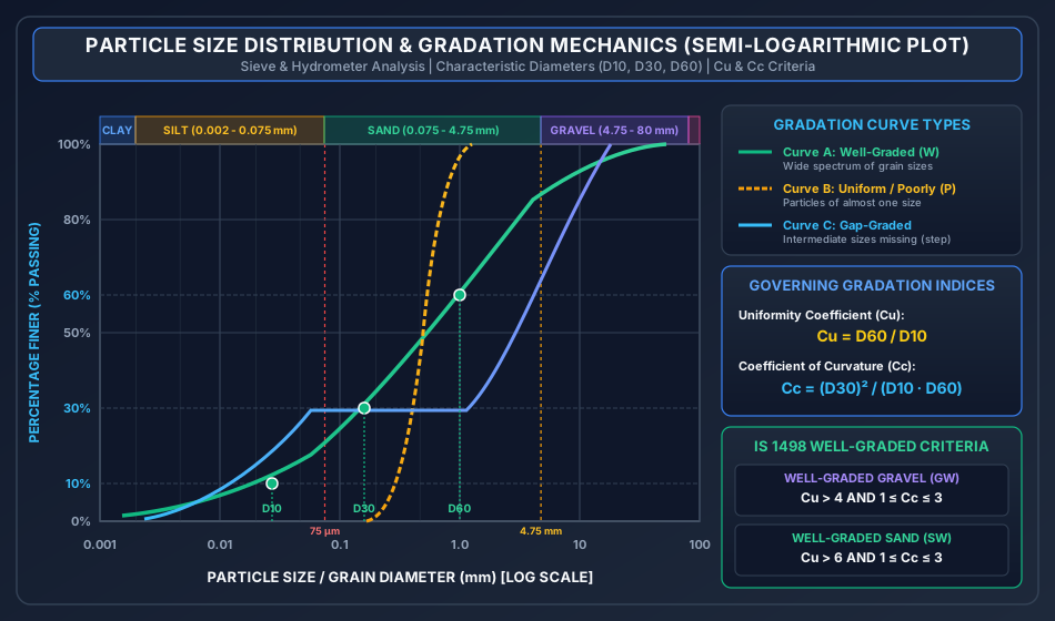
The grain size distribution curve plots Percentage Finer (, linear scale) versus Particle Diameter (, logarithmic scale). The logarithmic scale accommodates particle diameters spanning from to with equal visual clarity.
Characteristic Diameters:
- (Effective Size): Diameter corresponding to finer by weight. Hazen showed that the hydraulic permeability of clean filter sands correlates with ().
- : Diameter corresponding to finer by weight.
- : Diameter corresponding to finer by weight.
Gradation Shape Indices:
- Uniformity Coefficient ():
Measures the breadth or particle size range of the distribution:
- : Perfectly uniform soil (all grains of identical size; vertical curve).
- : Poorly graded / uniformly graded.
- (Gravel) or (Sand): Well-graded spanning a wide size spectrum.
- Coefficient of Curvature / Concavity ( or ):
Measures the geometric smoothness and absence of intermediate size gaps:
- For a well-graded soil: .
- If or : The soil is gap-graded (intermediate fractions missing, producing a flat step in the curve) or poorly graded.
| Gradation Classification | Curve Appearance on Semi-Log Plot | Criteria for IS 1498 Identification |
|---|---|---|
| Well-Graded Soil () | Smooth, wide, continuous S-shaped curve spanning multiple decades | Gravel: and Sand: and |
| Uniformly / Poorly Graded () | Steep, near-vertical curve over a narrow diameter band | Fails either the or criterion |
| Gap-Graded Soil | Stepped curve with a distinct horizontal plateau | Intermediate sizes absent; typically or |
4. Consistency of Cohesive Soils & Atterberg Limits
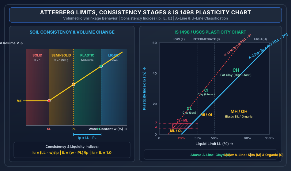
In 1911, the Swedish agricultural chemist Albert Atterberg established that as moisture is added to a fine-grained clay, it passes through four distinct mechanical consistency states:
           ◄────────────────── WATER CONTENT w INCREASING ──────────────────►
     ┌──────────────┬──────────────────┬──────────────────┬──────────────────┐
     │  SOLID STATE │ SEMI-SOLID STATE │  PLASTIC STATE   │   LIQUID STATE   │
     │              │                  │                  │                  │
     │ No volume    │ Volume expands   │ Soil is molded   │ Soil flows like  │
     │ change on    │ on wetting;      │ into shapes      │ a viscous slurry │
     │ drying (Vd)  │ cracks on drying │ without cracking │ under vibration  │
     └──────────────┴──────────────────┴──────────────────┴──────────────────┘
                    ▲                  ▲                  ▲
                    │                  │                  │
              SHRINKAGE LIMIT    PLASTIC LIMIT       LIQUID LIMIT
                   (SL)               (PL)               (LL)
4.1 The Fundamental Atterberg Limits
- Liquid Limit ( or ):
- The moisture content boundary between the plastic state and liquid state.
- At the liquid limit, all soils possess an identical, extremely small shear strength of approximately to ().
- Determination (Casagrande Apparatus, IS 2720 Part 5): Soil pat placed in a brass cup, divided with a standard Casagrande grooving tool (or ASTM tool for sandy soils) to an 11 mm wide base and 2 mm gap. The cup drops onto a hard rubber base at . The Liquid Limit is the water content at which the groove closes over a length of in exactly .
- Flow Curve & Flow Index (): Semi-logarithmic plot of moisture content () vs number of blows (, log scale): A high flow index indicates rapid shear strength loss with moisture addition.
- Cone Penetrometer Method: Modern Indian Standard preference: water content at which a standard polished cone of mass penetrates exactly into a soil pat in 5 seconds.
- Plastic Limit ( or ):
- The moisture content boundary between the semi-solid state and plastic state.
- Determination (IS 2720 Part 5): The water content at which the soil begins to crumble when rolled into continuous threads of () diameter.
- Shrinkage Limit ( or ):
- The maximum water content below which further moisture loss causes no further reduction in total soil volume.
- At , meniscus retreats into pores, air enters the voids (), and the soil volume stabilizes at constant dry pat volume .
- Determination (IS 2720 Part 6): A saturated soil pat of initial volume and mass is dried to constant mass and dry volume (measured via mercury displacement).
4.2 Derived Plasticity & Consistency Indices
| Index | Mathematical Formula | Physical & Practical Engineering Significance |
|---|---|---|
| Plasticity Index () | The numerical breadth of the plastic range. Directly proportional to clay mineral fraction and specific surface area. Non-plastic soils (sands): . Highly plastic montmorillonite: . | |
| Liquidity Index ( or ) | Quantifies the natural in-situ moisture state relative to plastic limits: • : Brittle semi-solid/solid (overconsolidated, hard stiff clays). • : Plastic state (normally consolidated clays). • : Fluid slurry; susceptible to spontaneous collapse upon shock (quick clays). |
|
| Consistency Index () | Invariant sum rule: . Measures in-situ stiffness against shear failure. represents hard/stiff crust. | |
| Toughness Index () | Measures the shear strength of clay at its plastic limit. For most natural clays, . If , the clay is friable and easily erodible at the plastic limit. | |
| Shrinkage Ratio () | Ratio of volume change (as % of dry volume) to moisture loss above shrinkage limit. Exactly equals the dry density ratio of the dried pat. | |
| Volumetric Shrinkage () | Total percentage volume reduction experienced by a soil element as its water content decreases from initial moisture down to the shrinkage limit. |
5. Soil Classification Systems (IS 1498:1970 & USCS)
The Indian Standard Soil Classification System (ISSCS, IS 1498:1970) is an extension of Casagrande's Unified Soil Classification System (USCS) tailored to subcontinental geology. It designates every soil type with a unique two-letter symbol:
        PRIMARY PREFIX (Soil Grain Type)          SECONDARY SUFFIX (Gradation / Plasticity)
        ────────────────────────────────          ─────────────────────────────────────────
        G : Gravel                                W : Well-graded (clean)
        S : Sand                                  P : Poorly graded (clean)
        M : Silt (Inorganic)                      M : Silty (contains silty fines > 12%)
        C : Clay (Inorganic)                      C : Clayey (contains clayey fines > 12%)
        O : Organic silt / clay                   L : Low compressibility (LL < 35%)
        Pt: Peat (Highly organic)                 I : Intermediate compressibility (35% ≤ LL ≤ 50%)
                                                  H : High compressibility (LL > 50%)
5.1 Primary Division Criteria
                                  OVERALL SOIL SAMPLE
                                           │
                     ┌─────────────────────┴─────────────────────┐
                     ▼                                           ▼
          [ COARSE-GRAINED SOILS ]                    [ FINE-GRAINED SOILS ]
          > 50% retained on 75 µm sieve               > 50% passes 75 µm sieve
                     │                                           │
          ┌──────────┴──────────┐                     ┌──────────┴──────────┐
          ▼                     ▼                     ▼                     ▼
       GRAVEL (G)            SAND (S)               CLAY (C)              SILT (M)
      > 50% coarse         > 50% coarse            Plots ABOVE           Plots BELOW
      retained on          passes 4.75 mm            A-Line                A-Line
      4.75 mm sieve
5.2 Coarse-Grained Classification Details (Gravels & Sands)
Based strictly on the percentage of fine particles passing :
- Fines (Clean Coarse Soils):
- Evaluated solely on and :
- (Well-graded Gravel): and .
- (Poorly graded Gravel): Fails or .
- (Well-graded Sand): and .
- (Poorly graded Sand): Fails or .
- Evaluated solely on and :
- Fines between and (Borderline Soils):
- Dual Symbols Required! Combines gradation and fines plasticity:
- Examples: , , , .
- Fines (Dirty Coarse Soils):
- Evaluated by plotting the fines fraction on the Atterberg Plasticity Chart:
- (Clayey Gravel) / (Clayey Sand): Fines plot above the A-Line ().
- (Silty Gravel) / (Silty Sand): Fines plot below the A-Line ().
- Evaluated by plotting the fines fraction on the Atterberg Plasticity Chart:
5.3 Fine-Grained Classification & The Plasticity Chart (IS 1498)
Fine-grained soils are classified by plotting Plasticity Index () against Liquid Limit ():
The A-Line:
- Above A-Line: Inorganic Clays ().
- Below A-Line: Inorganic Silts () and Organic Soils (). (Distinguished by oven drying: if drops by upon oven drying at , the soil is organic ).
The U-Line (Upper Limit Boundary):
- Represents the upper boundary of test data for all natural soils. Any test coordinate plotting above the U-line indicates laboratory testing or calculation error.
Compressibility Subdivisions:
- Low Compressibility (): ().
- Intermediate Compressibility (): (). (Note: USCS merges and into a single group; the group is an Indian Standard IS 1498 specialty).
- High Compressibility (): ().
The Dual Hatched Region ():
When the soil fines have:
The soil is classified with the dual symbol (Silty Clay of Low Plasticity).
6. Rigorous Analytical Derivations & Mathematical Proofs
6.1 Derivation 1: Terminal Settling Velocity from Stokes' Law
Proof: Consider a spherical soil grain of diameter falling through quiescent water under gravity:
- Submerged Gravitational Force ():
- Hydrodynamic Drag Force (): From Stokes' fluid mechanics solution for creeping laminar flow past a sphere ():
- Dynamic Terminal Equilibrium (): When terminal settling velocity is attained, acceleration is zero: Canceling and :
6.2 Derivation 2: Analytical Formula for Shrinkage Limit ()
Proof: Consider a saturated soil pat of initial moisture (), volume , and mass . As the pat dries from down to , it remains saturated (), and the volume loss equals the exact volume of water evaporated:
The mass of water evaporated during this transition:
The mass of water present at the shrinkage limit:
Dividing by dry solid mass :
Since :
Expressing in terms of Shrinkage Ratio () and Specific Gravity (): At the shrinkage limit, the soil pat is completely saturated with volume and solid mass :
Dividing both sides by :
Recall that Shrinkage Ratio . Substituting:
Multiplying through by :
7. Visual Vector Graphics & Engineering Schematics
7.1 Particle Size Distribution Curves & Gradation Mechanics
The semi-logarithmic chart below illustrates the size boundaries from clay to gravel, contrasting well-graded, uniformly graded, and gap-graded deposits, alongside characteristic diameter callouts:
7.2 Atterberg Limits & IS 1498 Plasticity Chart
The engineering schematic below illustrates the consistency volume-moisture relationship alongside the authoritative IS 1498 Plasticity Chart:
8. Laboratory Testing Procedures & Standards (IS 2720)
8.1 Sieve Analysis Protocol (IS 2720 Part 4)
- Apparatus: Riffle box sample divider, mechanical sieve shaker, standard brass sieves (), sensitive balance ( accuracy).
- Procedure: Dry sample weighed (). Sieve nested in decreasing order with pan at bottom. Shaken for 10 minutes. Mass retained on each sieve weighed.
- Calculations:
- Percentage retained on -th sieve: .
- Cumulative percentage retained: .
- Percentage finer (% passing): .
8.2 Casagrande Liquid Limit Test (IS 2720 Part 5)
- Apparatus: Mechanical cup with hard ebonite base, Casagrande and ASTM grooving tools, gauge block ().
- Groove Closure Criterion: The groove must close along the bottom over a continuous length of .
- Test Range: At least 4 trials distributed between and blows. The plot of vs is a straight line. is interpolated at .
9. Step-by-Step Pre-Calculated Numerical Examples
Problem 1: Complete Sieve Analysis, Gradation Parameters & Classification
Statement: A dry soil sample weighing was passed through a standard IS sieve stack. The masses retained on various sieves are tabulated below:
| Sieve Aperture Size | Mass Retained () |
|---|---|
| Pan |
- Calculate the percentage retained, cumulative percentage retained, and percentage finer for each sieve.
- Determine by semi-logarithmic interpolation the characteristic sizes , , and .
- Compute the Uniformity Coefficient () and Coefficient of Curvature ().
- Evaluate whether this sand can be classified as well-graded.
Detailed Step-by-Step Solution:
Step 1: Gradation Table Computation Total mass .
| Sieve (mm) | Mass Ret. (g) | % Retained | Cumulative % Retained | % Passing () |
|---|---|---|---|---|
| Pan |
Step 2: Logarithmic Interpolation of The semi-logarithmic interpolation formula between points and is:
-
(Interpolate between () and ()):
-
(Interpolate between () and ()):
-
(Interpolate between () and ()):
Step 3: Uniformity & Curvature Coefficients Uniformity coefficient:
Coefficient of curvature:
Step 4: Gradation Evaluation For a well-graded sand (), IS 1498 requires:
- (Satisfied)
- (Satisfied)
Problem 2: Atterberg Limits, Consistency Indices & Shrinkage Test
Statement: A cohesive clay sample has a liquid limit , a plastic limit , and an in-situ natural water content . In a laboratory shrinkage limit test, a saturated pat of this soil had an initial volume and an initial wet mass . After slow oven-drying to constant mass, the dry pat had a volume and a dry mass . Taking , determine:
- The plasticity index (), liquidity index (), and consistency index ().
- The initial water content of the shrinkage pat ().
- The shrinkage limit () of the soil.
- The shrinkage ratio () and specific gravity ().
- The volumetric shrinkage () when the soil dries from its in-situ moisture () to the shrinkage limit.
Detailed Step-by-Step Solution:
Step 1: Plasticity and Consistency Indices Plasticity Index:
Liquidity Index:
Consistency Index:
Verification Check: (Verified).
Step 2: Initial Water Content of Shrinkage Pat
Step 3: Shrinkage Limit ()
Step 4: Shrinkage Ratio () and Specific Gravity () Shrinkage Ratio:
Specific Gravity from shrinkage parameters:
Step 5: Volumetric Shrinkage ()
Problem 3: Multi-Stage Soil Classification as per IS 1498:1970
Statement: Comprehensive laboratory tests were performed on two soil samples, Soil X and Soil Y. The test results are summarized as follows:
| Parameter | Soil Sample X | Soil Sample Y |
|---|---|---|
| Passing IS Sieve | ||
| Passing IS Sieve | ||
| Liquid Limit () of Fines | ||
| Plastic Limit () of Fines | ||
| Sand Fraction | — | |
| Sand Fraction | — | |
| Sand Fraction | — |
Classify both Soil X and Soil Y according to IS 1498:1970, giving step-by-step reasoning for all symbol selections.
Detailed Step-by-Step Solution:
Classification of Soil X:
- Coarse vs Fine-Grained Division:
- Percentage passing .
- Percentage retained on .
- Soil X is a COARSE-GRAINED SOIL.
- Gravel vs Sand Division:
- Coarse fraction of total soil.
- Retained on (Gravel fraction).
- Passing and retained on (Sand fraction).
- Since Sand () Gravel (), the primary soil component is SAND ().
- Fines Fraction Analysis ():
- The fines fraction is exactly (the borderline threshold between clean and dirty sands).
- Per IS 1498, soils with fines between and require DUAL SYMBOLS.
- Gradation of Sand Fraction: The sand matrix is Well-Graded ().
- Plasticity of Fines:
- Fines Plasticity Index: .
- A-Line Plasticity Index:
- Since , the fines plot above the A-Line, designating them as Clayey ().
- Dual Symbol Assignment:
Classification of Soil Y:
- Coarse vs Fine-Grained Division:
- Percentage passing .
- Soil Y is a FINE-GRAINED SOIL.
- Compressibility Subdivision:
- Liquid Limit .
- Since , the soil has Intermediate Compressibility () as per IS 1498.
- Position Relative to A-Line on Plasticity Chart:
- Soil Plasticity Index: .
- A-Line Plasticity Index:
- Since , the soil coordinates plot strictly above the A-Line.
- Soils plotting above the A-Line are Inorganic Clays ().
- Group Symbol Assignment: Combining Clay () with Intermediate Compressibility ():
10. Common Exam Traps, Failure Modes & Field Gotchas
[!WARNING]
The 5 Critical Traps in Soil Gradation & Classification
- The Sand vs. Gravel Denominator Trap:
- When evaluating whether a coarse soil is Sand () or Gravel (), compare the gravel fraction against the sand fraction as a percentage of the coarse fraction alone, NOT the total soil!
- Rule: If coarse fraction is of total, and gravel is , sand is . Gravel is of coarse fraction GRAVEL (), even though gravel is of the total soil!
- The Borderline Fines Dual Symbol Rule:
- Students often write a single symbol ( or ) for a soil with fines.
- Fatal Error: IS 1498 and USCS mandate dual symbols for ().
- The Dual Hatched Zone Trap:
- If a fine-grained soil has and plots above the A-line (), students often classify it simply as .
- Trap: Any soil in this narrow hatched zone must be classified with the dual symbol .
- USCS vs. IS 1498 Intermediate Compressibility () Trap:
- In USCS, there are only two plasticity subdivisions: Low () and High ().
- In Indian Standard (IS 1498), there are three subdivisions: Low (), Intermediate (), and High ().
- In Indian exams (GATE, ESE, SSC JE), always use the three-tier system!
- Stokes' Law Fines Lower Limit Fallacy:
- Stokes' law fails for particles smaller than (), NOT because of turbulence, but because of Brownian motion (random thermal kinetic bombardment by fluid molecules preventing gravity settling).
11. Multi-Exam Targeted Practice Questions
Question 1 (GATE CE Computational)
A fine-grained soil has a liquid limit and a plastic limit . As per IS 1498:1970, the group symbol of the soil is:
- (A)
- (B)
- (C)
- (D)
Correct Answer: (B)
Step-by-Step Derivation:
- High Compressibility ().
- .
- A-line value: .
- Since , the soil plots above the A-line Clay ().
- Combining: (Inorganic Clay of High Plasticity).
Question 2 (UPSC ESE Conventional - 10 Marks)
Explain with neat sketches the Casagrande Liquid Limit test. Derive the equation of the flow index () and discuss the significance of the toughness index ().
Model Answer Outline:
- Apparatus: Casagrande brass cup dropping onto hard rubber base at 2 drops/sec.
- Grooving Tools: Casagrande tool (for clayey soils, 2 mm bottom width, 11 mm top, 8 mm depth) and ASTM tool (for sandy soils).
- Definition: Water content corresponding to 25 blows for a 12 mm closure along groove bottom.
- Flow Curve & Flow Index Derivation: Plotting vs yields a straight line: represents the rate of shear strength degradation with water content.
- Toughness Index: At the liquid limit, all soils have equal minimal shear strength (). As moisture drops to the plastic limit, shear strength increases by a factor proportional to . Hence, directly measures the shearing strength of the soil at its plastic limit. For typical soils, . Soils with crumble rapidly under shear.
Question 3 (SSC JE Rapid Recall)
A soil has a liquid limit of and a plastic limit of . The plasticity index is:
- (A)
- (B)
- (C)
- (D) Non-plastic
Correct Answer: (A)
Explanation: .
Question 4 (State AE Objective)
For a well-graded gravel, the values of and must satisfy:
- (A) and
- (B) and
- (C) and
- (D) and
Correct Answer: (A) and
Explanation: By IS 1498 / USCS, gravel requires , while sand requires , with both requiring .
Question 5 (RRB JE Technical)
The meniscus correction in hydrometer reading is always:
- (A) Positive
- (B) Negative
- (C) Zero
- (D) Positive or negative depending on temperature
Correct Answer: (A) Positive
Explanation: The meniscus curves upward around the hydrometer stem. In an opaque soil suspension, the reading must be taken at the upper rim of the meniscus, which reads a smaller number (lower density). Hence, the meniscus correction is always added ().
12. Reference Standards & Authoritative Handbooks
- Bureau of Indian Standards:
- IS 1498: 1970 – Classification and Identification of Soils for General Engineering Purposes.
- IS 2720 (Part 4): 1985 – Grain Size Analysis.
- IS 2720 (Part 5): 1985 – Determination of Liquid and Plastic Limits.
- IS 2720 (Part 6): 1972 – Determination of Shrinkage Factors.
- Authoritative Textbooks:
- Karl Terzaghi, Ralph B. Peck, and Gholamreza Mesri, Soil Mechanics in Engineering Practice, 3rd ed., John Wiley & Sons.
- Gopal Ranjan and A. S. R. Rao, Basic and Applied Soil Mechanics, New Age International.
- B. C. Punmia, Ashok Kumar Jain, and Arun Kumar Jain, Soil Mechanics and Foundations, 16th ed., Laxmi Publications.
- Arthur Casagrande, Classification and Identification of Soils, Transactions of ASCE, Vol. 113, 1948.