Railway Engineering — Permanent Way, Track Geometry, Cant Dynamics, Points & Crossings, and Maintenance Standards
In this chapter (1 topics)
On this page
- 1. Module Overview & Technical Architecture
- 2. Governing Formulae, Empirical Relations & Code Provisions
- 2.1 Track Gauges on Indian Railways (IRPWM Standards)
- 2.2 Equilibrium Cant (Superelevation) & Dynamic Equilibrium
- 2.3 Indian Railways Cant, Deficiency & Excess Limits (IRPWM Table of Standards)
- 2.4 Safe Maximum Speed on Transitioned Curves (Indian Railways Empirical Equations)
- 3. Step-by-Step Analytical Derivations & Mechanisms
- 3.1 Derivation of Equilibrium Cant Formula
- 3.2 Wheel Coning & Tilting of Rails (Adzing) Mechanics
- 3.3 Cole's Turnout Geometry Derivation
- 3.4 Minimum Depth of Ballast Cushion (db)
- 4. Permanent Way Elements & Technical Specifications
- 4.1 Rail Metallurgy & Heavy-Haul Standardization (IRS T-12 / UIC 860)
- 4.2 Permissible Rail Wear Limits Before Renewal (IRPWM Chapter III)
- 4.3 Sleepers: Classification, Performance & Sleeper Density
- 5. Creep of Rails, Joint Mechanics & Welded Rails
- 5.1 Creep of Rails: Definition, Phenomenon & Causes
- 5.2 Permissible Creep Limits & Remedial Interventions
- 5.3 Welded Track Hierarchy (SWR, LWR, CWR)
- 6. Geometric Design of Railway Track
- 6.1 Gradients & Grade Compensation on Curves
- 6.2 Transition Curves & Cant Gradient
- 7. Points & Crossings, Turnout Geometry & Interlocking
- 7.1 Anatomy & Mechanical Components of a Turnout
- 7.2 Negative Superelevation on Turnouts
- 8. Track Maintenance, Inspection & High-Speed Standards
- 8.1 Track Quality Indices & Recording Cars
- 8.2 Mechanized Maintenance (Tamping & Deep Screening)
- 9. Embedded Technical Visualizations & Diagrams
- 9.1 Permanent Way Embankment Cross-Section & Wheel Coning Mechanics
- 9.2 Turnout Anatomy, Points & Crossings Geometry and Cant Dynamics
- 10. Worked Analytical & Design Numerical Problems
- Problem 1: Equilibrium Cant, Cant Excess, and Permissible Speed on Broad Gauge Curve
- Problem 2: Complete Geometry of a 1 in 12 Broad Gauge Turnout (Cole's Method)
- Problem 3: Sleeper Density, Spacing, and Minimum Depth of Ballast Cushion
- 11. Cross-Exam Synthesis Matrix
- 12. Common Failure Modes, Site Diagnostics & Forensic Engineering
- 12.1 Track Buckling in Continuous Welded Rails (CWR)
- 12.2 Rolling Contact Fatigue (RCF) & Rail Flaw Types
- 13. Practice Problems & Exam Drill Questions
- Question 1 (GATE Style — NAT)
- Question 2 (UPSC ESE Style — Conceptual Multiple Choice)
- Question 3 (SSC JE / RRB JE Style — Quick Recall)
- 14. Comprehensive Technical Reference & Cross-Topic Linkages
- Inter-Topic Knowledge Mapping
- Standard Code References
1. Module Overview & Technical Architecture
Railway Engineering governs the planning, design, construction, operation, and maintenance of guided ground transportation infrastructure. Unlike highway pavements where pneumatic rubber tires distribute wheel loads over relatively flexible pavement structures with free vehicular steering degrees of freedom, a railway track structure (termed the Permanent Way) constitutes a specialized, semi-elastic guided structural system. Lateral guidance is enforced exclusively through steel wheel-rail contact mechanics, conicity of wheel treads, and wheel flanges.
The permanent way comprises a layered load-transfer composite:
- Rails: Longitudinal steel beams that carry concentrated moving wheel loads (axle loads up to 22.5 to 25.0 tonnes on Indian Railways Broad Gauge), provide an ultra-smooth running surface with minimal rolling resistance (), and serve as electrical conductors for track circuits in automated signalling.
- Fastenings & Elastic Pads: Resilient fasteners (e.g., Elastic Rail Clips / Pandrol clips, grooved rubber sole pads) that clamp the rails to sleepers with designed toe loads (), attenuating high-frequency wheel impact vibrations and insulating track circuits.
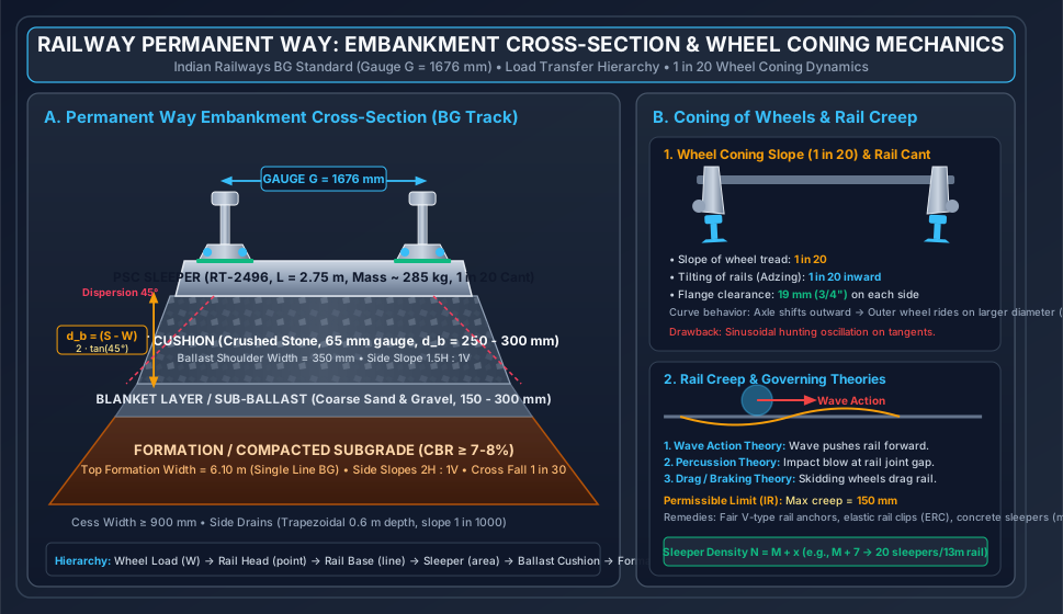
- Sleepers (Ties): Transverse structural beams (predominantly Monoblock Prestressed Concrete Sleepers, PSC RT-2496) that maintain the track gauge, anchor the rails at a 1 in 20 inward tilt, and distribute concentrated wheel reactions over the ballast bed.
- Ballast Cushion: Angular, crushed rock aggregate ( gauge) that provides uniform resilient support, transfers stresses safely to the sub-ballast, allows rapid lateral and longitudinal water drainage, and resists lateral/longitudinal track displacement under thermal stresses and braking forces.
- Sub-Ballast / Blanket & Formation (Subgrade): Coarse sand-gravel blanket layer () overlying the compacted subgrade that prevents subgrade soil pumping, attenuates dynamic stress below the subgrade bearing capacity (), and ensures long-term slope and embankment stability.
Wheel Axle Load (25 t) ──► Point Contact on Rail Head (Hertzian Contact Stress ~ 800 - 1200 MPa)
         │
         ▼
Rail Section (Bending & Shear Transfer) ──► Distributed Line Load on Rail Seat
         │
         ▼
Elastomeric Pad & Sleeper Bearing Area (Compressive Stress ~ 1.5 - 2.5 MPa)
         │
         ▼
Ballast Bed (Pyramidal 45° Stress Dispersion ~ 0.3 - 0.5 MPa)
         │
         ▼
Blanket / Sub-ballast & Compacted Formation Subgrade (~ 0.08 - 0.12 MPa)
2. Governing Formulae, Empirical Relations & Code Provisions
2.1 Track Gauges on Indian Railways (IRPWM Standards)
The track gauge is defined as the minimum clear distance between the running inner faces of the two rails measured at a depth of below the top surface of the rail head.
| Gauge System | Symbol | Clear Distance () | Dynamic Gauge ( for Cant) | Remarks & Modern Usage |
|---|---|---|---|---|
| Broad Gauge (BG) | Standard | () | () | Universal standard (Project Unigauge); of IR route-km |
| Metre Gauge (MG) | MG | () | Phase-wise converted to BG; retained in heritage corridors | |
| Narrow Gauge (NG) | NG | () & | / | Mountain railways (Kalka-Shimla, Darjeeling Himalayan Railway) |
2.2 Equilibrium Cant (Superelevation) & Dynamic Equilibrium
On a horizontal curve of radius (metres), a railway vehicle travelling at speed () is subjected to an outward centrifugal force . To neutralize lateral flange thrust and achieve equal wheel reactions on both inner and outer rails, the outer rail is elevated above the inner rail by an equilibrium cant ():
Where:
- = Equilibrium cant (metres; multiply by for millimetres).
- = Dynamic gauge (centre-to-centre of rail heads: for BG, for MG, for NG).
- = Vehicle speed ().
- = Curve radius (). On Indian Railways, degree of curve is based on a standard () chord: (metres).
2.3 Indian Railways Cant, Deficiency & Excess Limits (IRPWM Table of Standards)
| Parameter | Broad Gauge (BG) | Metre Gauge (MG) | Narrow Gauge () |
|---|---|---|---|
| Maximum Permissible Cant () | (General routes) (Special permission, Group A routes) |
||
| Permissible Cant Deficiency () | () (, nominated routes) |
||
| Permissible Cant Excess () | |||
| Rate of Cant Deficiency Change |
2.4 Safe Maximum Speed on Transitioned Curves (Indian Railways Empirical Equations)
For Broad Gauge transitioned curves, the maximum permissible speed is the minimum of:
- Speed based on Theoretical Equilibrium Cant + Cant Deficiency:
- Indian Railways Empirical Formula (Martin's Formula modified by Railway Board):
- For transitioned curves ():
- For high-speed routes (, Group A routes):
- Speed governed by Rate of Cant Deficiency / Gain ( check):
3. Step-by-Step Analytical Derivations & Mechanisms
3.1 Derivation of Equilibrium Cant Formula
Consider a railway wagon of mass and weight traversing a circular curve of radius at constant speed (). The outer rail is raised by height over gauge width , tilting the axle plane by angle .
           Centrifugal Force P = (W * v^2) / (g * R)
                     ◄───────────● (C.G.)
                                 │
                                 │ Weight W = mg
                                 ▼
                     /|
                    / |
    Track Plane    /  | e (Cant)
   (Width G)      / θ |
                 /____|
- Resolving forces parallel to the inclined rail top surface:
- For dynamic equilibrium (no lateral centrifugal thrust on wheel flanges, equal vertical reactions on both rails):
- Since the cant angle is small ():
- Equating both expressions:
- Converting () to () where , and taking :
3.2 Wheel Coning & Tilting of Rails (Adzing) Mechanics
Railway wheels are not cylindrical; they are manufactured with a conical taper of 1 in 20 sloping outward from the wheel flange towards the outer edge.
Dynamic Action of Coning:
- On Tangent (Straight) Track: If an external lateral disturbance shifts the axle towards the left rail:
- The left wheel tread contacts the rail head at a larger rolling diameter ().
- The right wheel tread contacts at a smaller rolling diameter ().
- In one axle rotation, the left wheel traverses distance , exceeding the right wheel distance .
- This differential rolling distance steers the wheelset back towards the track centreline, providing automatic, self-centering lateral stability without flange rubbing.
- Side-effect: This restoring action induces a periodic, sinusoidal oscillation known as Hunting Oscillation (), attenuated by bogie dampers and track gauge tightening.
- On Curved Track: Centrifugal force pushes the axle outward. The outer wheel rides on its maximum tread diameter near the root of the flange, while the inner wheel rides on its smaller diameter. The difference in circumference accommodates the extra path length of the outer circular curve (), preventing longitudinal wheel slippage.
- Tilting of Rails (1 in 20 Inward Cant): Because conical wheels exert inclined resultant contact forces, placing flat-bottomed rails horizontally causes severe, eccentric, point wear on the inner edge of the rail head. To ensure centric vertical wheel-load transmission along the rail web axis, rails are tilted inward at 1 in 20. This is accomplished by:
- Providing inclined canted rail seats in modern PSC sleepers.
- Using tapered canted bearing plates on steel/cast iron sleepers.
- Adzing (planing at 1 in 20 inclination) wooden sleepers under the rail seat.
3.3 Cole's Turnout Geometry Derivation
In a standard turnout, the lead curve branches from the straight stock rail. Under Cole's Method (adopted universally in Indian practice):
- The crossing angle is defined by the number , where (or ).
- The lead curve is assumed circular from the tangent point at the toe of the switch to the Theoretical Nose of Crossing (TNC).
Stock Rail (Straight):   ─────────────────────────────────────────────────────────────
Toe of Switch:           ▲               Lead of Crossing (L)                ▲ (TNC)
                         │◄─────────────────────────────────────────────────►│
                         │             Curve Lead (CL = 2 * G * N)           │
                         │◄──────────────────────────────────────────────────│
                         │◄────────►│
                       Switch Lead (SL = √(2*R*d))
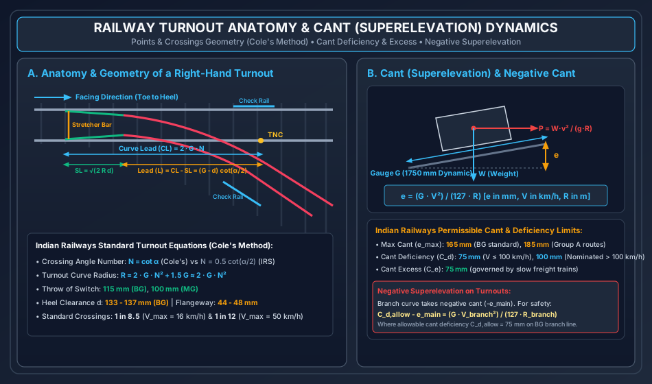
- Curve Lead (): The longitudinal distance from the toe of the switch to the theoretical nose of crossing:
- Radius of Curve (): From circle geometry, .
- Switch Lead (): The distance from the toe of the switch to the heel of the switch where the clearance is (heel divergence):
- Lead of Crossing (): The distance from the heel of switch to the theoretical nose of crossing:
3.4 Minimum Depth of Ballast Cushion ()
The primary functional duty of ballast is to disperse the high compressive pressure beneath the sleeper seat down to a safe, uniform stress below the bearing capacity of the subgrade.
- Let = sleeper centre-to-centre spacing ().
- Let = width of sleeper bottom surface ().
- Assuming ballast aggregate disperses load at an internal distribution angle of : To prevent stress overlap or gaps where ballast remains unloaded, the adjacent 45° dispersion envelopes must just meet at the formation top:
4. Permanent Way Elements & Technical Specifications
4.1 Rail Metallurgy & Heavy-Haul Standardization (IRS T-12 / UIC 860)
Indian Railways has phased out 90 lb () and older 75 lb rails on broad gauge trunk routes, adopting standard flat-bottomed sections:
| Feature | 52 kg/m Rail | 60 kg/m Rail (UIC 60) | 68 kg/m (Heavy Haul / DFC) |
|---|---|---|---|
| Cross-Sectional Area | |||
| Total Height () | |||
| Foot Width () | |||
| Web Thickness () | |||
| Moment of Inertia () | |||
| Section Modulus () | |||
| Steel Grade / UTS | 90 UTS () Micro-alloyed () |
90 UTS & 110 UTS Head Hardened (HH) | 110 UTS Head Hardened (340-390 BHN) |
| Standard Lengths | (standard single), (welded panels) | / / (Jindal / SAIL) | Flash-butt welded strings |
4.2 Permissible Rail Wear Limits Before Renewal (IRPWM Chapter III)
- Vertical Wear: Measured along the central vertical axis of the head:
- For rails: .
- For rails: .
- Lateral Wear: Measured at below the top of the rail head on curves:
- Group A & B routes: .
- Group C & D routes: .
- Total Cross-Sectional Area Loss: of initial cross-sectional area.
4.3 Sleepers: Classification, Performance & Sleeper Density
Where:
- = Length of one rail in metres ( for BG, for MG).
- = Arbitrary integer factor depending on traffic density, axle load, and speed (typically on Indian Railways).
- Example: .
| Sleeper Type | Material & Compressive Strength | Service Life | Weight | Advantages & Operational Limitations |
|---|---|---|---|---|
| PSC Monoblock (RT-2496) | Prestressed Concrete (), 18-HT strands | Heavy mass provides maximum lateral track resistance against buckling in LWR/CWR; excellent track circuit insulation with composite liners; susceptible to impact fracture during derailment. | ||
| Steel Trough | Pressed structural steel plate ( thick) | Lightweight, easy to handle, excellent scrap value; susceptible to severe corrosion in coastal/saline soil; requires insulating pads for track circuiting. | ||
| Cast Iron (CST-9) | Cast iron plates with central steel tie bar | Good scrap value; brittle, cannot withstand modern heavy axle/high-speed dynamic loads; entirely obsolete on trunk lines. | ||
| Wooden (Sal, Teak, Deodar) | Hardwood / Softwood treated with creosote oil | Unmatched shock and vibration damping; ideal for bridge girders and complex turnouts; prone to rotting, termite decay, and fire. |
5. Creep of Rails, Joint Mechanics & Welded Rails
5.1 Creep of Rails: Definition, Phenomenon & Causes
Creep is the longitudinal, progressive movement of rails relative to the sleepers over time. Creep is predominantly observed in the direction of traffic on double-track lines, and in the direction of heavier haul/dominant downward gradient on single-track lines.
Mechanics of Creep Generation:
- Wave Action Theory: Under moving wheel loads, the continuous rail acts as an elastic beam on an elastic foundation, deflecting downward under each wheel and developing a reverse, elevated wave-like bulge immediately ahead of the rolling wheel. As wheels roll forward, they continuously shove this crest forward, dragging the rail longitudinally.
- Percussion Theory: At every rail joint gap ( to expansion gap), the wheel rolls off the end of the trailing rail and delivers a high-energy oblique impact blow against the receiving end of the facing rail, pushing it forward in the direction of travel.
- Braking / Drag Theory: When trains apply brakes, the skidding frictional reaction between the brake blocks, locked wheels, and rail surface drags the rails in the direction of movement. Conversely, when locomotives accelerate, driving wheels exert a backward reaction.
       Wheel Direction ──►
              (●)
    ─────────/   \────────────  <- Rail deflection wave
   Negative       Deflection
    Hogging         Basin
5.2 Permissible Creep Limits & Remedial Interventions
- Permissible Tolerance (IRPWM): Creep in excess of is unacceptable and must be immediately adjusted.
- Consequences of Uncontrolled Creep:
- Closing of joint gaps during hot summer afternoons leads to explosive lateral track buckling.
- Wide opening of joints in freezing winter causes sheared fishbolts and broken fishplates.
- Distortion of points and crossings, misaligning switch blades and jamming interlocking stretchers.
- Anti-Creep Remedies:
- Installation of Rail Anchors (e.g., Fair V-type spring anchors clipped to the rail foot bearing tightly against sleeper faces; minimum anchors per rail).
- Adoption of modern Elastic Rail Clips (ERC Mark-III/Mark-V) maintaining toe loads .
- Conversion of fishplated joints into continuous welded track.
5.3 Welded Track Hierarchy (SWR, LWR, CWR)
Depending on the degree of thermal restraint, rail continuity is categorized into:
- Short Welded Rails (SWR): Typically 3-rail panels () welded together, with conventional mechanical expansion joints at ends. The entire panel contracts and expands thermally.
- Long Welded Rails (LWR): A welded rail length where the central longitudinal portion remains completely stationary (immobile) under seasonal thermal cycles (). The thermal stresses () in the central section are completely resisted by longitudinal ballast bed resistance (). Only the breathing lengths () at either end expand and contract: Switch Expansion Joints (SEJ) are provided at the boundaries to accommodate breathing movement ().
- Continuous Welded Rails (CWR): An LWR that extends uninterrupted through station yards, points, and crossings over distances of multiple kilometres (spanning block sections).
6. Geometric Design of Railway Track
6.1 Gradients & Grade Compensation on Curves
Gradients are introduced to negotiate elevation differences between stations:
- Ruling Gradient: The maximum gradient permitted on a railway section that governs the maximum locomotive hauling capacity.
- Plains: ().
- Rolling/Hilly: ().
- Pusher / Helper Gradient: A steeper grade () in ghat sections where an auxiliary banking/pusher locomotive is attached to assist the lead engine.
- Momentum Gradient: A steeper grade positioned immediately after a descending valley, where train kinetic energy overcomes the extra grade resistance.
Grade Compensation on Curves:
When a curve coincides with a grade, the total resistance equals grade resistance plus curve resistance ( on BG). To ensure the total resistance does not exceed the ruling gradient resistance:
Code Reductions per Degree of Curve ():
- Broad Gauge (BG): per degree ().
- Metre Gauge (MG): per degree ().
- Narrow Gauge (NG): per degree ().
6.2 Transition Curves & Cant Gradient
Transition curves are inserted between a tangent and circular curve to gradually introduce curvature ( from to ) and cant ( to ), preventing sudden lateral acceleration lurch ().
- Ideal Transition Curve Profile: Cubic Parabola () for small deflection angles, or Clothoid Spiral.
- Length of Transition Curve (): Indian Railways prescribes as the maximum of:
- Rate of cant deficiency gain ():
- Rate of cant gain ():
- Maximum cant gradient ( on normal routes; for high-speed):
7. Points & Crossings, Turnout Geometry & Interlocking
7.1 Anatomy & Mechanical Components of a Turnout
A standard turnout is an assembly of track components that diverts rolling stock from one track line to an adjacent diverging line without interruption.
       Toe of Switch
             │
Stock Rail ──┼───────────────────────────────────────────────────────────── (Main Track)
             │ \  Tongue Rail
             │  \
             │   \  Lead Rail             Throat    TNC      Check Rail
             │    \─────────────────────────\───────●───────── (Branch Track)
             │                               \ Wing  \
             │                                \ Rail  \
             │                                 ───────●─────── Check Rail
- Points / Switch Assembly:
- Stock Rails: Continuous main track rails against which tongue rails nest.
- Tongue Rails (Switch Blades): Tapered, movable machining-profile rails. The thin tapered forward tip is the Toe, and the fixed rear end is the Heel.
- Stretcher Bars: Steel tie-bars connecting both tongue rails at the toe to ensure simultaneous movement when actuated by switch motors.
- Throw of Switch: The lateral distance through which the tongue rail toe travels between open and closed positions:
- Broad Gauge: ().
- Metre Gauge: ().
- Heel Clearance (): The clear lateral gap between the gauge face of the stock rail and the back of the tongue rail at the heel ( for BG).
- Crossing Assembly:
- Provides wheel flange passage where the outer branch rail intersects the inner main rail.
- Vee Piece: Formed by the union of the Point Rail and Splice Rail.
- Theoretical Nose of Crossing (TNC): The mathematical point of intersection of the gauge lines.
- Actual Nose of Crossing (ANC): The physical, blunted nose (ground back by to a thickness of ) to prevent wheel impact chipping.
- Wing Rails: Flared rails that guide wheel tread over the crossing gap.
- Check Rails (Guard Rails): Rails mounted parallel to the opposite running rails that engage the wheel inner backface, preventing wheel flanges from striking or climbing the nose of crossing. Flangeway clearance .
7.2 Negative Superelevation on Turnouts
When a branch line diverges from a curved main line in the opposite direction, the outer rail of the main line is elevated by cant to satisfy main line speeds. However, this same outer main rail becomes the inner rail of the diverging turnout curve. Consequently, the branch line experiences an unfavorable Negative Cant ():
To prevent derailment due to excessive overturning outward moment on the branch line:
- The allowable cant deficiency on the branch line ( on BG) must absorb both the negative cant and the centrifugal requirement:
- The permissible speed on the branch track () is strictly restricted by:
8. Track Maintenance, Inspection & High-Speed Standards
8.1 Track Quality Indices & Recording Cars
Indian Railways deploys high-speed Track Recording Cars (TRC) utilizing contactless optical/laser gyro sensors to compute the Track Recording Index (TRN) and Track Quality Index (TQI).
- Track Tolerances Monitored:
- Gauge Variation: Deviation from nominal ( on straight high-speed lines, on curves).
- Unevenness (Twist): Variation in cant measured over a base of (should not exceed ).
- Alignment: Horizontal chord deviation over a chord ().
- Cross-Level / Superelevation Error: .
8.2 Mechanized Maintenance (Tamping & Deep Screening)
- Tamping Machines (Plasser Duomatic / 08-32U): Hydraulically insert vibrating tamping tines beneath sleeper seats, lifting and slewing the track back to its theoretical design vertical profile and alignment while consolidating ballast aggregate under high-frequency squeeze vibration ().
- Ballast Cleaning Machines (BCM): Continuously excavate foul ballast aggregate, screen out silt, pulverized dust, and particles , and return clean aggregate to the track bed, restoring track drainage.
9. Embedded Technical Visualizations & Diagrams
9.1 Permanent Way Embankment Cross-Section & Wheel Coning Mechanics
The cross-sectional anatomy of a broad gauge railway embankment, detailing the hierarchy of load distribution from rail to subgrade, combined with the 1 in 20 wheel coning geometry and rail creep theories, is presented below.
9.2 Turnout Anatomy, Points & Crossings Geometry and Cant Dynamics
The complete geometry of a right-hand turnout (Cole's Method), showing switch leads, crossing leads, check rails, and the free-body diagram governing dynamic equilibrium cant and negative superelevation, is illustrated below.
10. Worked Analytical & Design Numerical Problems
Problem 1: Equilibrium Cant, Cant Excess, and Permissible Speed on Broad Gauge Curve
Statement: A horizontal curve is situated on a Broad Gauge (, dynamic gauge ) trunk line. The line carries mixed traffic:
- Weighted average / equilibrium speed of traffic = .
- Maximum sanctioned speed for fast passenger express trains = .
- Speed of slow goods trains negotiating the curve = .
Calculate:
- Radius of the curve ().
- Theoretical equilibrium cant for the average speed.
- Actual cant to be provided () satisfying Indian Railways standards for cant deficiency () and cant excess ().
- Maximum permissible speed () on the curve, checking both cant deficiency limits and the Railway Board empirical formula for transitioned curves.
Analytical Solution:
Step 1: Radius of Curve () Using standard Indian Railways chord definition ( chord):
Step 2: Theoretical Cant Calculations Using the dynamic cant formula :
- For Equilibrium Speed ():
- For Maximum Fast Train Speed ():
- For Slow Goods Train Speed ():
Step 3: Determining Actual Cant to be Provided ()
- Governed by Slow Freight Trains (Cant Excess Limit ): When slow trains crawl at , an excessively high outer rail causes wheel loads to concentrate on the inner rail, risking track shift or rail crushing.
- Governed by Fast Passenger Trains (Cant Deficiency Limit ): For fast passenger comfort at : Observation: To permit without exceeding , an actual cant of at least would be needed. However, the absolute maximum permissible cant on BG is (and cant excess for goods trains caps it at ). Therefore, the slow goods train cant excess strictly governs the maximum allowable actual cant: (Note: This satisfies ).
Step 4: Maximum Permissible Speed () Since is lower than , the fast trains cannot be permitted at . We compute the allowable safe speed:
- From Maximum Permissible Cant Deficiency ():
- From Indian Railways Empirical Formula for Transitioned Curves ():
- Adopted Safe Speed Limit:
Problem 2: Complete Geometry of a 1 in 12 Broad Gauge Turnout (Cole's Method)
Statement: Calculate the complete geometric dimensions for a turnout on a Broad Gauge track () using Cole's Method. The heel clearance () is provided as (). Determine:
- Crossing angle () in degrees, minutes, and seconds.
- Radius of the turnout lead curve ().
- Curve Lead ().
- Switch Lead ().
- Lead of Crossing ().
Analytical Solution:
Step 1: Crossing Angle () In Cole's Method, the crossing number is defined along the cotangent:
Converting to degrees, minutes, and seconds:
- Whole degrees:
- Minutes:
- Seconds:
Step 2: Radius of Turnout Curve () Under Cole's formulation, taking track gauge :
Step 3: Curve Lead () The curve lead is the distance from the toe of the switch to the Theoretical Nose of Crossing (TNC):
Step 4: Switch Lead () The switch lead is the distance from the toe of switch to the heel of switch where divergence is :
Step 5: Lead of Crossing () The lead of crossing represents the distance from the heel of switch to the TNC:
Problem 3: Sleeper Density, Spacing, and Minimum Depth of Ballast Cushion
Statement: A Broad Gauge track section with standard rails has a specified sleeper density of . The PSC sleepers used have a bottom bearing width of . Assuming the wheel load disperses through the ballast aggregate at an angle of to the vertical, determine:
- Number of sleepers per rail panel and total sleepers required per kilometre of track.
- Centre-to-centre spacing of sleepers ().
- Minimum theoretical depth of clean ballast cushion () beneath the sleeper seat.
Analytical Solution:
Step 1: Number of Sleepers & Track Density Given rail length and density formula where :
For () of track:
Step 2: Centre-to-Centre Sleeper Spacing () Assuming uniform spacing along the rail:
Step 3: Minimum Depth of Ballast Cushion () Using the 45° dispersion equation:
Given , sleeper width , and :
Engineering Note: On Indian Railways, while is the theoretical minimum cushion depth for this spacing, the IRPWM mandates a standard minimum cushion of for all BG routes carrying LWR/CWR, and for heavy-haul routes (25 t axle load / Dedicated Freight Corridors) to account for aggregate degradation and mechanized tamping tolerances.
11. Cross-Exam Synthesis Matrix
| Exam | High-Frequency Conceptual Focus | Typical Calculation Types | Priority Traps & Critical Nuances |
|---|---|---|---|
| GATE CE | • Equilibrium cant derivation () • Cant deficiency & excess governing checks • Speed limits on transitioned curves • Ballast cushion depth formula () |
• Numerical Answer Type (NAT) cant and speed limits • Cole's turnout geometry () • Grade compensation calculations |
• Dynamic gauge () must be used in the formula, NOT nominal gauge () • Degree of curve in IR is defined by chord () • Do not confuse cant excess with cant deficiency. |
| UPSC ESE | • Full derivation of Cole's Turnout Geometry • LWR breathing length & thermal stress analysis • Track modulus () • Mechanized maintenance & track recording |
• Conventional 15-mark design of turnouts and curves • Negative superelevation numericals • Sleeper density and ballast volume estimation |
• Always check both slow and fast speeds before declaring actual cant • Remember to state code limits (, ) • Mention adzing of sleepers when explaining wheel coning. |
| SSC JE / RRB JE | • Standard gauges (BG , MG , NG ) • Wheel coning taper () and tilting () • Throw of switch ( BG) • Creep theories and rail anchor usage |
• Direct formula substitution for , , or • Sleeper density • Grade compensation ( BG) |
• Do not forget flangeway clearance () vs throw of switch () • Rail weight defined per unit length (, NOT per piece) • Creep permissible limit is . |
| State AE / PSU | • Types of rail sections (Flat footed vs Bull headed) • Fishplate specifications and joint clearance • Ruling gradient values across terrains • Turnout numbers ( vs ) |
• Ruling gradient with curve compensation • Number of sleepers in a given length • Maximum permissible speed Martin formula |
• Bull-headed rails require cast iron chairs and wooden/steel keys; flat-footed rails do not • On turnouts, speed is strictly restricted to on loops. |
12. Common Failure Modes, Site Diagnostics & Forensic Engineering
12.1 Track Buckling in Continuous Welded Rails (CWR)
- Failure Phenomenon: Explosive, instantaneous lateral displacement of the track panel (often several hundred millimetres) during peak summer afternoon heat, resulting in catastrophic derailment.
- Root Cause & Forensic Diagnosis:
- Compressive thermal stress , where is the stress-free destressing temperature.
- Deficiency in ballast shoulder width () or loose, unconsolidated crib ballast following improper maintenance.
- Unchecked creep accumulating high compressive stresses in local pockets.
- Site Remediation:
- Regular de-stressing of LWR track using hydraulic rail tensors to lock in the target neutral temperature ().
- Maintenance of full ballast shoulder width of with shoulder compaction.
12.2 Rolling Contact Fatigue (RCF) & Rail Flaw Types
- Head Checking & Gauge Corner Cracking (GCC): High shear stress and cyclic plastic deformation at the wheel-rail gauge corner induce micro-cracks sloping at to the surface.
- Shatter Cracks & Transverse Fissures: Internal metallurgical hydrogen embrittlement generating progressive internal transverse fatigue fractures that propagate unseen until catastrophic rail breakage under dynamic train impact.
- Ultrasonic Flaw Detection (USFD): Periodic non-destructive testing using 0°, 70°, and 37° piezoelectric ultrasonic probes to detect internal flaws before critical propagation.
13. Practice Problems & Exam Drill Questions
Question 1 (GATE Style — NAT)
On a Broad Gauge track, a horizontal curve of radius is provided with a transition curve. If the maximum speed of fast trains is and the actual cant provided on the track is , determine the cant deficiency experienced by the fast trains in . (Dynamic gauge ).
- Answer:
- Explanation: Then Cant Deficiency . Note: Since , this speed exceeds the permissible limit on IR and requires speed restriction!
Question 2 (UPSC ESE Style — Conceptual Multiple Choice)
Which of the following statements regarding Railway Engineering on Indian Railways is/are INCORRECT?
- The dynamic gauge used in the superelevation formula is for Broad Gauge.
- The maximum permissible cant excess on Broad Gauge track is .
- In Cole's Method for turnouts, the radius of the curve is approximately .
- The rate of grade compensation on Broad Gauge curves is per degree of curve.
- Options: (a) 1 and 3 only (b) 2 only (c) 2 and 4 only (d) 3 only
- Correct Answer: (b) 2 only
- Explanation: The maximum permissible cant excess () on Indian Railways Broad Gauge track is (not ). Statements 1, 3, and 4 are entirely correct.
Question 3 (SSC JE / RRB JE Style — Quick Recall)
If the ruling gradient on a BG railway section is and a horizontal curve is located on this section, the compensated gradient is:
- Calculation:
- Ruling gradient .
- Curve compensation for BG .
- Compensated gradient .
14. Comprehensive Technical Reference & Cross-Topic Linkages
Inter-Topic Knowledge Mapping
- Upstream Linkages:
SOM-01toSOM-04: Elastic beam on elastic foundation (Winkler foundation model for rail bending and depression).GEOTECH-05&06: Stress distribution in soil (Boussinesq theory applied to ballast-formation contact) and subgrade compaction.
- Concurrent & Downstream Linkages:
TRANS-01: Geometric design principles (stopping distance vs braking distance, horizontal curvature).TRANS-04: Mechanistic-empirical layered pavement concepts mirrored in ballast-blanket-formation design.TRANS-06: Airport and harbor engineering (intermodal freight logistics, rail terminal container sidings).
Standard Code References
- IRPWM (2020): Indian Railways Permanent Way Manual, Ministry of Railways, Government of India.
- IRS Track Manual: Standard Specifications for Rails, Sleepers, Turnouts, Fasteners and Ballast.
- UIC Code 714R / 774-3R: Classification and Track-Bridge Interaction Standards, International Union of Railways.
- IS 3986 / IRS T-12: Specifications for Flat Bottom Railway Rails.