Pavement Design: Flexible (IRC 37:2018 Mechanistic-Empirical) & Rigid Pavement (IRC 58:2015 Westergaard)
In this chapter (1 topics)
On this page
- 1. Title & Authoritative References
- 2. Prerequisites & Learning Objectives
- Prerequisites
- Learning Objectives
- 3. Structural Mechanics: Flexible vs. Rigid Pavements
- 3.1 Fundamental Comparison
- 4. Flexible Pavement Design per IRC 37:2018
- 4.1 Structural Layer Configuration
- 4.2 Traffic Estimation in Cumulative Standard Axles (CSA / MSA)
- 4.3 Subgrade Resilient Modulus (MR)
- 4.4 Mechanistic-Empirical Failure Transfer Functions
- 5. Pavement Structural Evaluation & Overlay Design
- 5.1 Benkelman Beam Deflection (BBD) Technique (IRC: 81-1997)
- 6. Rigid Pavement Design per IRC 58:2015
- 6.1 Westergaard's Theory & Foundation Assumptions
- 6.2 Westergaard Wheel Load Stress Formulations
- 7. Temperature Stresses & Critical Stress Combinations
- 7.1 Temperature Warping Stresses (σt)
- 7.2 Subgrade Frictional Stresses (σf)
- 7.3 Critical Design Stress Combinations (IRC: 58-2015)
- 8. Concrete Joint Engineering (IRC: 58-2015)
- 8.1 Transverse Contraction Joints
- 8.2 Transverse Expansion Joints
- 8.3 Longitudinal Joints & Tie Bars
- 9. Analytical Derivations
- Derivation 1: Radius of Relative Stiffness (l)
- Derivation 2: Subgrade Frictional Stress (σf)
- 10. Solved Numerical Example 1: Flexible Pavement Traffic & Modulus (IRC 37)
- Problem Statement
- Step-by-Step Analytical Solution
- 11. Solved Numerical Example 2: Rigid Pavement Westergaard Wheel Stresses
- Problem Statement
- Step-by-Step Analytical Solution
- 12. Solved Numerical Example 3: Thermal Stresses & Critical Stress Combinations
- Problem Statement
- Step-by-Step Analytical Solution
- 13. Common Misconceptions & Exam Traps
- 1. Vehicle Damage Factor (VDF) Fourth Power Law
- 2. The Resisting Section Cutoff (1.724 h)
- 3. Dowel Bars vs. Tie Bars
- 4. Warping Stress Direction: Day vs. Night
- 14. Quick Revision Summary & Formula Sheet
- 15. References & Standard Codes
1. Title & Authoritative References
- Indian Roads Congress Standard Codes:
- IRC: 37-2018: Guidelines for the Design of Flexible Pavements (Fourth Revision)
- IRC: 58-2015: Guidelines for the Design of Plain Jointed Rigid Pavements for Highways (Fourth Revision)
- IRC: 81-1997: Guidelines for Strengthening of Flexible Road Pavements Using Benkelman Beam Deflection Technique
- IRC: 115-2014: Guidelines for Structural Evaluation and Overlay Design of Flexible Pavements Using Falling Weight Deflectometer (FWD)
- IRC: SP: 76-2015: Guidelines for Conventional and Thin White-Topping
- MoRTH (5th Revision): Specifications for Road and Bridge Works, Sections 400, 500, and 600.
- Academic & International Authorities:
- Westergaard, H.M. (1926, 1948), Stresses in Concrete Pavements Computed by Theoretical Analysis, Public Roads & Proceedings of Highway Research Board.
- Bradbury, R.D. (1938), Reinforced Concrete Pavements, Wire Reinforcement Institute, Washington D.C.
- Huang, Y.H., Pavement Analysis and Design, 2nd Edition, Pearson Education.
- Yoder, E.J. and Witczak, M.W., Principles of Pavement Design, 2nd Edition, John Wiley & Sons.
- AASHTO, Guide for Design of Pavement Structures, American Association of State Highway and Transportation Officials.
2. Prerequisites & Learning Objectives
Prerequisites
- Solid Mechanics & Elasticity: Bending of thin plates, bi-harmonic differential equations (), plane strain elasticity, Winkler foundation springs.
- Statistics & Growth Projections: Geometric compounding series, probability distributions, variance and standard deviation.
- Viscoelastic Materials: Dynamic resilient modulus, temperature susceptibility, creep and fatigue phenomena.
Learning Objectives
- Contrast the structural load-distribution mechanisms, stress dissipation profiles, and failure criteria of flexible versus rigid pavements.
- Execute design traffic modeling in Cumulative Standard Axles (CSA / MSA) using the Fourth Power Law Vehicle Damage Factor (VDF) per IRC: 37-2018.
- Compute the effective subgrade resilient modulus () and evaluate pavement mechanistic-empirical strain limits: bottom tensile strain () for fatigue cracking and top subgrade vertical strain () for rutting.
- Derive Westergaard's radius of relative stiffness () and equivalent radius of resisting section (); compute wheel load stresses at Interior (), Edge (), and Corner () positions.
- Formulate thermal warping stresses () via Bradbury coefficients and subgrade frictional stresses (); assemble critical seasonal edge and corner stress combinations.
- Design concrete pavement expansion joints, contraction dummy grooves, smooth dowel bars, and deformed tie bars in strict compliance with IRC: 58-2015.
3. Structural Mechanics: Flexible vs. Rigid Pavements
Pavements are engineered multi-layered structural systems designed to distribute concentrated vehicular wheel loads safely to the underlying subgrade bed without exceeding the allowable resilient or shear strain capacities of any constituent layer.
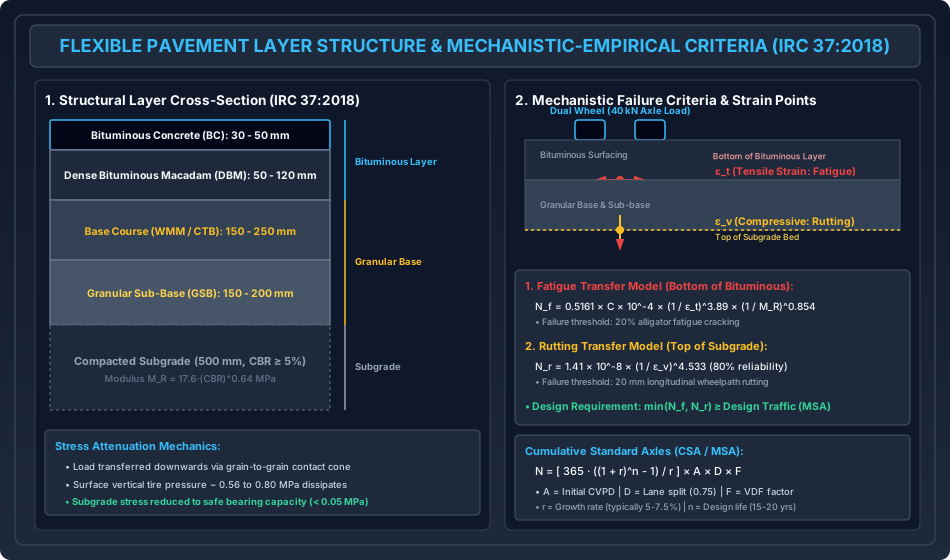
3.1 Fundamental Comparison
| Structural Feature | Flexible Pavement (Bituminous) | Rigid Pavement (Cement Concrete) |
|---|---|---|
| Load Distribution Mechanism | Grain-to-grain contact; stress dissipates downward through a truncated conical pyramid ( distribution) | Slab flexural action (Beam/Plate bending); load distributed over a very wide area by structural slab rigidity |
| Structural Rigidity () | Very low flexural rigidity; bends under wheel loads | Extremely high flexural rigidity () |
| Subgrade Strength Sensitivity | Highly sensitive to subgrade CBR; low CBR demands significantly thicker granular base layers | Less sensitive to subgrade variations; slab bridges minor localized soft spots |
| Temperature Effects | Softens at high temperatures (rutting); hardens at low temperatures (thermal fatigue cracking) | Subject to severe thermal warping stresses due to vertical temperature gradients () |
| Critical Stress Location | Tensile strain at bottom of asphalt; vertical compressive strain at top of subgrade | Tensile flexural stress at bottom (mid-day) or top (midnight) of concrete slab |
| Service Life & Maintenance | Design life: ; requires periodic resurfacing/overlays every | Design life: ; low routine maintenance, higher initial capital cost |
4. Flexible Pavement Design per IRC 37:2018
IRC: 37-2018 establishes a Mechanistic-Empirical (M-E) design framework. Traffic loads and climatic variables are converted into mechanical stresses and strains via multi-layer linear elastic theory (e.g., IITPAVE software), which are then related to field pavement performance using empirical failure transfer functions.
4.1 Structural Layer Configuration
A standard heavy-duty flexible pavement consists of five distinct layers:
- Surface Wearing Course: Bituminous Concrete (BC, ), utilizing VG-40 or Polymer Modified Bitumen (PMB) to provide skid resistance, surface drainage, and abrasion resistance.
- Binder Course: Dense Bituminous Macadam (DBM, ), providing primary structural flexural strength.
- Granular Base Course: Wet Mix Macadam (WMM, ) or Cement Treated Base (CTB).
- Granular Sub-Base (GSB): Crushed stone/gravel (), serving as a structural cushion and capillary cutoff layer.
- Compacted Subgrade: top thickness of compacted select earth ( Modified Proctor MDD, minimum design ).
4.2 Traffic Estimation in Cumulative Standard Axles (CSA / MSA)
Design traffic () represents the total cumulative number of equivalent standard axles ( single axle load with dual wheels) expected during the pavement design life:
where:
- = Initial traffic (commercial vehicles per day, CVPD): where is commercial traffic volume during survey, is annual traffic growth rate (), and is the construction completion delay period in years.
- = Design Life: (Expressways/NH), (heavy arterial corridors).
- = Lateral / Directional Distribution Factor:
- Single-lane road (two-way traffic): (all traffic concentrated in single lane).
- Two-lane undivided single carriageway: of total two-way CVPD (or per direction).
- Four-lane divided dual carriageway: of CVPD in each directional carriageway.
- Six-lane divided dual carriageway: of directional CVPD.
- = Vehicle Damage Factor (VDF / Equivalency Factor): The multiplier converting an average commercial vehicle into equivalent standard axles. Derived from the AASHO Road Test Fourth Power Law:
Standard Reference Axles:
- Single Axle with Single Wheels: ()
- Single Axle with Dual Wheels: ()
- Tandem Axle with Dual Wheels: ()
- Tridem Axle with Dual Wheels: ()
4.3 Subgrade Resilient Modulus ()
The elastic modulus of the subgrade soil under repeated transient vehicular pulses:
- For :
- For :
4.4 Mechanistic-Empirical Failure Transfer Functions
The pavement trial cross-section must be checked against two primary distress failure criteria:
1. Fatigue Cracking Criterion
Repeated tensile flexural straining at the bottom of the bituminous layer causes microscopic bottom-up alligator cracking:
where is the maximum horizontal tensile strain at the bottom of the DBM layer, is the resilient modulus of the bituminous layer at design pavement temperature (), and is a volumetric adjustment factor.
- Permissible Limit: .
2. Subgrade Rutting Criterion
Permanent accumulation of unrecoverable vertical compressive strains at the subgrade top leads to longitudinal wheelpath depression:
where is the vertical compressive strain at the subgrade surface.
- Permissible Limit: .
5. Pavement Structural Evaluation & Overlay Design
When an existing flexible pavement deteriorates under service traffic, non-destructive deflection testing evaluates the structural rebound capacity of the pavement-subgrade system to size structural overlays.
5.1 Benkelman Beam Deflection (BBD) Technique (IRC: 81-1997)
The Benkelman Beam utilizes a pivoted beam with a probe arm placed between the dual rear wheels of a standard testing truck loaded to ( rear axle load) with tire inflation pressure of ().
Analytical Procedure:
- Rebound Deflection (): where is initial dial reading under dual wheels, and is final reading when the truck drives away ( accounts for beam lever ratio ).
- Mean and Standard Deviation:
- Characteristic Deflection (): Accounts for statistical variability in the pavement section:
- Environmental Corrections: where is temperature correction ( per below standard ), and is subgrade moisture correction factor based on subgrade plasticity and soil field moisture content.
- Overlay Thickness Design ():
6. Rigid Pavement Design per IRC 58:2015
Rigid pavements consist of high-strength Pavement Quality Concrete (PQC, minimum flexural strength ) slabs constructed over a Dry Lean Concrete (DLC) sub-base.
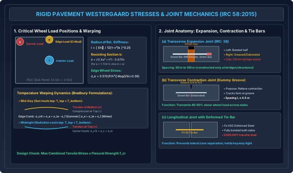
6.1 Westergaard's Theory & Foundation Assumptions
H.M. Westergaard analyzed a homogeneous, isotropic, elastic concrete slab resting continuously on a Winkler subgrade (dense liquid foundation where upward subgrade reaction is directly proportional to localized slab deflection : ).
1. Radius of Relative Stiffness ()
The fundamental parameter governing the structural stiffness of the concrete slab relative to the subgrade:
where:
- = Modulus of elasticity of concrete ()
- = Slab thickness ()
- = Poisson's ratio of concrete ()
- = Modulus of subgrade reaction ( or )
2. Equivalent Radius of Resisting Section ()
Westergaard recognized that directly under a concentrated wheel load, ordinary thin plate bending theory yields infinite shear stresses. To account for local three-dimensional shear deformation:
- If contact radius :
- If contact radius :
where is the circular tire contact radius ().
6.2 Westergaard Wheel Load Stress Formulations
1. Interior Loading ():
Wheel load applied at the central interior zone of the slab away from edges:
2. Edge Loading ():
Wheel load applied at the longitudinal joint edge with wheel tangent to the edge. This generates the highest flexural tensile stress in the pavement:
3. Corner Loading ():
Wheel load applied at the intersection of two transverse and longitudinal joints. Acts as an unsupported cantilever:
7. Temperature Stresses & Critical Stress Combinations
Concrete slabs experience continuous dimensional changes from diurnal and seasonal ambient temperature variations.
7.1 Temperature Warping Stresses ()
Caused by vertical temperature differentials () between the top and bottom slab surfaces. Formulated by R.D. Bradbury:
where is the thermal expansion coefficient of concrete (), and is Bradbury's warping coefficient derived from the ratio (slab length to radius of relative stiffness).
- Diurnal Behavior:
- Day Warping (Summer/Winter Mid-Day): Sun heats top surface (). Slab curls convex upward. The weight of the slab resists curling, inducing tensile stress at the bottom of the slab and compression at the top.
- Night Warping (Midnight): Radiation cools top surface (). Slab curls concave upward. Edges and corners lift off the subgrade, inducing tensile stress at the top of the slab.
7.2 Subgrade Frictional Stresses ()
Caused by overall seasonal temperature drops (). As the slab contracts uniformly toward its center, frictional resistance between the slab underside and the sub-base opposes motion:
where is unit weight of concrete (), is slab length between contraction joints, and is coefficient of subgrade friction ( for granular sub-base, for rough DLC). Frictional stress produces uniform axial tension across the entire slab cross-section.
7.3 Critical Design Stress Combinations (IRC: 58-2015)
To ensure structural safety, the maximum combined tensile stress must be evaluated at two critical positions:
-
Critical Edge Stress (Mid-Day / Daytime Peak): Wheel load stress at edge () plus daytime bottom warping tension ():
- Summer Mid-Day: Slab expands, subgrade friction produces compression:
- Winter Mid-Day: Slab contracts, subgrade friction produces tension:
(Winter mid-day yields the absolute maximum tensile stress at the bottom of the slab).
-
Critical Corner Stress (Midnight / Nighttime Peak): Wheel load stress at corner () plus nighttime top warping tension ():
(Note: Subgrade friction is negligible at free corners).
- Statutory Design Requirement:
8. Concrete Joint Engineering (IRC: 58-2015)
Joints relieve internal expansion, contraction, and warping stresses, preventing uncontrolled random cracking.
8.1 Transverse Contraction Joints
Spaced closely at to limit warping and frictional stresses.
- Constructed as a "dummy groove" sawn into the hardened concrete to a depth of to ().
- Sawn groove creates a weakened vertical plane where the contraction crack forms cleanly underneath.
- Dowel Bars: Plain, round, smooth mild steel bars ( dia, length) spaced at across the joint. Half the bar is debonded (coated with grease or plastic sleeve) to allow free longitudinal sliding while transferring of shear wheel loads across the joint.
8.2 Transverse Expansion Joints
Provide room for unrestricted longitudinal expansion during peak summer, preventing slab blow-up buckling.
- Standard gap width: , filled with compressible premolded joint filler board (fiberboard or cork) and sealed with polyurethane/silicone sealant.
- Fitted with smooth dowel bars equipped with a metal expansion cap on the debonded half containing a compressible sponge/cotton plug to permit sliding without jamming.
- Modern IRC: 58 practice omits expansion joints along open roadways, restricting them strictly to bridge abutments, culvert interfaces, and permanent structures.
8.3 Longitudinal Joints & Tie Bars
Constructed along the lane boundary to prevent warping cracking across wide multi-lane slabs and stop lanes from separating laterally.
- Tie Bars (HYSD / Fe 500 Deformed Steel): Diameter , length , spaced at .
- Unlike dowel bars, tie bars are fully bonded into concrete on both sides.
- Tie bars DO NOT transfer wheel loads; they act purely in tension to resist subgrade lateral sliding friction: where is distance from joint to free edge, and is allowable steel tensile stress.
9. Analytical Derivations
Derivation 1: Radius of Relative Stiffness ()
Consider an elastic thin concrete plate of thickness resting on a Winkler subgrade with reaction modulus . The governing bi-harmonic plate bending differential equation under distributed load is:
where is the flexural rigidity of the plate:
and is the upward subgrade reaction. Under free plate deformation ():
Introducing a characteristic dimensional scaling length such that :
Substituting flexural rigidity :
Derivation 2: Subgrade Frictional Stress ()
Consider a rectangular slab of length , width , thickness , and unit weight . During seasonal temperature drop, the slab contracts symmetrically toward its center line (). At distance from the centerline, the contracting movement is resisted by uniform frictional shear stress at the subgrade interface. Equating the internal tensile force at cross-section to the cumulative frictional drag from the free edge ():
Dividing both sides by cross-sectional area :
The maximum frictional tensile stress occurs at the slab center ():
10. Solved Numerical Example 1: Flexible Pavement Traffic & Modulus (IRC 37)
Problem Statement
A two-lane undivided National Highway is planned for a design life of .
- Initial commercial traffic volume from traffic census: at completion of construction.
- Annual compound traffic growth rate: .
- Design Vehicle Damage Factor: .
- Directional / Lateral distribution factor per IRC: 37-2018: .
- Laboratory soaked CBR of the subgrade soil: .
- Compute the cumulative standard axles (CSA) in Million Standard Axles (MSA) over the design life.
- Determine the design effective subgrade resilient modulus ().
Step-by-Step Analytical Solution
-
Traffic Compounding Growth Factor:
-
Cumulative Standard Axles ():
-
Subgrade Resilient Modulus (): Since , use IRC: 37 power formulation:
11. Solved Numerical Example 2: Rigid Pavement Westergaard Wheel Stresses
Problem Statement
A concrete pavement slab has thickness .
- Modulus of elasticity of concrete: .
- Poisson's ratio: .
- Modulus of subgrade reaction: .
- Design wheel load: , tire contact pressure .
- Determine the radius of circular tire contact area ().
- Compute the radius of relative stiffness of the slab ().
- Evaluate the equivalent radius of resisting section ().
- Calculate the wheel load flexural stresses at the Edge () and Corner ().
Step-by-Step Analytical Solution
-
Contact Radius ():
-
Radius of Relative Stiffness ():
-
Equivalent Radius of Resisting Section (): Check threshold ratio:
Since :
-
Westergaard Stresses:
- Edge Stress ():
- Corner Stress ():
12. Solved Numerical Example 3: Thermal Stresses & Critical Stress Combinations
Problem Statement
For the pavement slab in Example 2:
- Slab panel length between contraction joints: .
- Thermal expansion coefficient: .
- Summer maximum temperature differential: .
- Bradbury's edge warping coefficient: .
- Coefficient of subgrade friction: ; Unit weight of concrete: .
- Characteristic 28-day flexural strength of concrete: ().
- Compute the edge temperature warping stress ().
- Compute the seasonal subgrade frictional stress ().
- Determine the critical combined edge stress for Summer Mid-Day and Winter Mid-Day. Check structural safety.
Step-by-Step Analytical Solution
-
Edge Warping Stress ():
-
Subgrade Frictional Stress ():
-
Critical Combined Edge Stresses: From Example 2, edge wheel load stress .
- Case A: Summer Mid-Day (Bottom of Slab in Tension):
- Case B: Winter Mid-Day (Bottom of Slab in Tension):
-
Flexural Capacity Check:
The pavement slab provides a safety factor of against bottom flexural cracking under combined vehicular and environmental extremes.
13. Common Misconceptions & Exam Traps
[!WARNING]
1. Vehicle Damage Factor (VDF) Fourth Power Law
- VDF scales with the fourth power of the axle load ratio, NOT linearly:
- An overloaded single axle ( legal load) does not cause damage; it inflicts the fatigue damage of a standard axle!
[!WARNING]
2. The Resisting Section Cutoff ()
- In Westergaard's stress equations, applies strictly when .
- If , thin plate theory holds cleanly and . Never blindly evaluate the square root expression without verifying .
[!WARNING]
3. Dowel Bars vs. Tie Bars
- Dowel Bars: Placed across transverse joints. Smooth, debonded on one side; design function is shear load transfer across adjacent slabs while allowing longitudinal sliding.
- Tie Bars: Placed across longitudinal joints. Deformed (HYSD), fully bonded; DO NOT transfer shear load; design function is purely tying slabs laterally against subgrade friction.
[!WARNING]
4. Warping Stress Direction: Day vs. Night
- Daytime Mid-Day: Surface expands slab hogs (convex up) Tension at bottom. Adds directly to bottom wheel load tensile stress at the edge.
- Nighttime Midnight: Surface contracts slab sags (concave up) Tension at top. Adds directly to top wheel load tensile stress at the corner.
14. Quick Revision Summary & Formula Sheet
+---------------------------------------------------------------------------------------------------+
| PAVEMENT DESIGN FORMULA SHEET (IRC 37:2018 / IRC 58:2015)                                         |
+---------------------------------------------------------------------------------------------------+
| 1. Flexible Pavement Design (IRC: 37-2018):                                                       |
|    - Design Traffic (CSA/MSA): N = [ 365 * ((1 + r)^n - 1) / r ] * A * D * F                      |
|      * Two-lane single carriageway: D = 0.75 | Four-lane divided: D = 0.75                        |
|    - Vehicle Damage Factor: VDF = SUM[ (Actual Axle / Standard 80 kN Axle)^4 ]                    |
|    - Subgrade Resilient Modulus:                                                                  |
|      * For CBR <= 5%: M_R = 10 * CBR (MPa)                                                        |
|      * For CBR > 5%:  M_R = 17.6 * (CBR)^0.64 (MPa)                                               |
|    - Fatigue Model: N_f = 0.5161 * C * 10^-4 * (1 / eps_t)^3.89 * (1 / M_R)^0.854                |
|    - Rutting Model: N_r = 1.41 * 10^-8 * (1 / eps_v)^4.533                                        |
+---------------------------------------------------------------------------------------------------+
| 2. Rigid Pavement Mechanics (IRC: 58-2015):                                                       |
|    - Radius of Relative Stiffness: l = [ (E * h^3) / (12 * (1 - nu^2) * k) ]^0.25                 |
|    - Resisting Section Radius:     b = sqrt(1.6 a^2 + h^2) - 0.675 h  (if a < 1.724 h)            |
|                                    b = a                              (if a >= 1.724 h)           |
|    - Interior Wheel Stress:        sigma_i = (0.316 P / h^2) * [ 4 log10(l / b) + 1.069 ]         |
|    - Edge Wheel Stress:            sigma_e = (0.572 P / h^2) * [ 4 log10(l / b) + 0.359 ]         |
|    - Corner Wheel Stress:          sigma_c = (3 P / h^2) * [ 1 - ((a * sqrt(2)) / l)^0.6 ]        |
+---------------------------------------------------------------------------------------------------+
| 3. Temperature & Frictional Stresses:                                                             |
|    - Edge Warping Stress:   sigma_te = (C_x * E * alpha_t * Delta_T) / 2                          |
|    - Subgrade Friction:     sigma_f  = gamma_c * (L / 2) * f                                      |
|    - Summer Mid-Day Comb:   sigma_crit = sigma_e + sigma_te - sigma_f                             |
|    - Winter Mid-Day Comb:   sigma_crit = sigma_e + sigma_te + sigma_f  (Absolute Maximum Peak)   |
|    - Midnight Corner Comb:  sigma_crit = sigma_c + sigma_tc                                       |
+---------------------------------------------------------------------------------------------------+
| 4. Joint Engineering:                                                                             |
|    - Contraction Spacing:   L <= 4.5 m | Dummy Groove depth = h/4 to h/3                          |
|    - Expansion Gap:         Delta = 20-25 mm | Dowel bar debonded with cap                        |
|    - Tie Bar Area (Steel):  A_st = (W * b' * f) / S_st  (HYSD deformed, fully bonded)             |
+---------------------------------------------------------------------------------------------------+
15. References & Standard Codes
- Indian Roads Congress (IRC):
- IRC: 37-2018: Guidelines for the Design of Flexible Pavements (4th Revision), New Delhi.
- IRC: 58-2015: Guidelines for the Design of Plain Jointed Rigid Pavements (4th Revision), New Delhi.
- IRC: 81-1997: Guidelines for Strengthening of Flexible Road Pavements, New Delhi.
- Ministry of Road Transport and Highways (MoRTH):
- Specifications for Road and Bridge Works (5th Revision), Indian Roads Congress, 2013.
- Primary Textbooks:
- Huang, Y.H., Pavement Analysis and Design, 2nd Edition, Prentice Hall.
- Khanna, S.K., Justo, C.E.G., and Veeraragavan, A., Highway Engineering, 10th Ed., Nem Chand & Bros.