Traffic Engineering: Flow Theory, Capacity & LOS, Signal Design (Webster & IRC), Intersections
In this chapter (1 topics)
On this page
- 1. Title & Authoritative References
- 2. Prerequisites & Learning Objectives
- Prerequisites
- Learning Objectives
- 3. Fundamental Traffic Stream Characteristics
- 3.1 Primary Microscopic and Macroscopic Variables
- 3.2 The Fundamental Hydrodynamic Traffic Equation
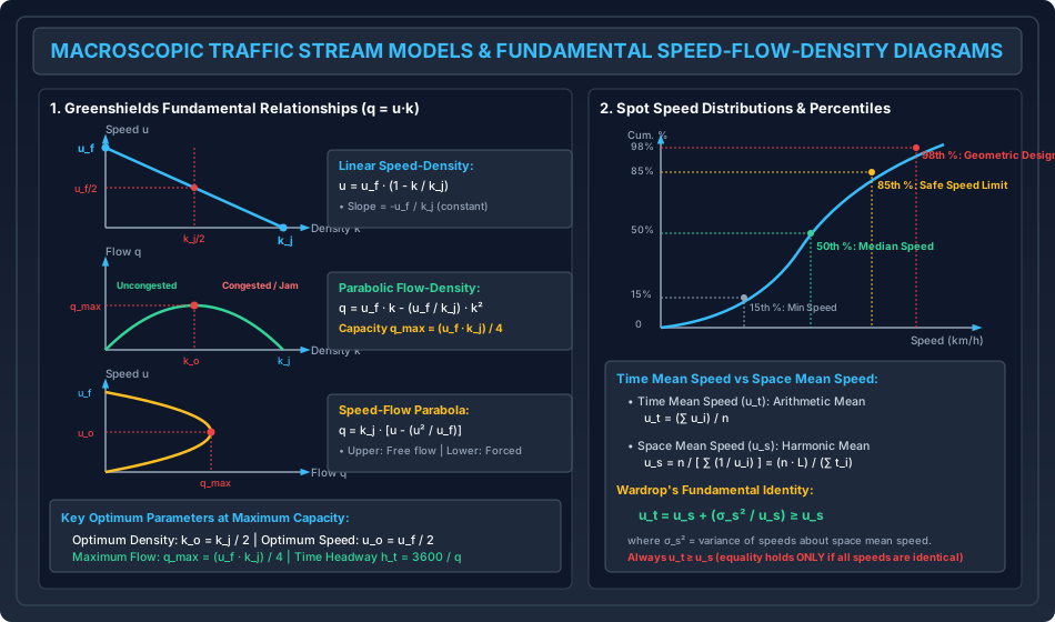
- 3.3 Macroscopic Speed-Density-Flow Models
- 4. Traffic Studies & Speed Analysis
- 4.1 Time Mean Speed (ut) vs. Space Mean Speed (us)
- 4.2 Wardrop's Fundamental Identity
- 4.3 Speed Percentiles and Engineering Significance
- 4.4 Passenger Car Units (PCU / PCE)
- 5. Roadway Capacity & Level of Service (LOS)
- 5.1 Hierarchical Definitions of Capacity
- 5.2 Level of Service (LOS) Concepts
- 6. Traffic Signal Design
- 6.1 Signal Terminology & Timing Dynamics
- 6.2 Webster's Method for Optimum Cycle Length
- 6.3 IRC: 93 Signal Design Method
- 6.4 The Dilemma Zone Problem
- 7. Intersections & Rotary Design
- 7.1 At-Grade Intersections
- 7.2 Rotary (Roundabout) Design Mechanics
- 8. Analytical Derivations
- Derivation 1: Theoretical Capacity in Greenshields Model
- Derivation 2: Wardrop's Inequality (ut ≥ us)
- 9. Solved Numerical Example 1: Traffic Flow & Speed Modeling
- Problem Statement
- Step-by-Step Analytical Solution
- 10. Solved Numerical Example 2: Signal Design by Webster's Method
- Problem Statement
- Step-by-Step Analytical Solution
- 11. Solved Numerical Example 3: Rotary Roundabout Design
- Problem Statement
- Step-by-Step Analytical Solution
- 12. Common Misconceptions & Exam Traps
- 1. Time Mean Speed vs. Space Mean Speed in Flow Calculations
- 2. The qmax Coordinates in Greenshields Model
- 3. Lost Time in Webster's Formula (L)
- 4. Weaving Ratio in Roundabout Sizing (p)
- 13. Quick Revision Summary & Formula Sheet
- 14. References & Standard Codes
1. Title & Authoritative References
- Indian Roads Congress Standard Codes:
- IRC: 106-1990: Guidelines for Capacity of Urban Roads in Plain Areas
- IRC: 64-1990: Guidelines for Capacity of Roads in Rural Areas
- IRC: 93-1985: Guidelines on Suitable Design of Traffic Signals
- IRC: 65-2017: Guidelines for Planning and Design of Roundabouts (First Revision)
- IRC: SP: 41-1994: Guidelines on the Design of At-Grade Intersections in Rural & Urban Areas
- IRC: SP: 90-2010: Manual for Safety in Road Design
- CSIR-CRRI (2017): Indian Highway Capacity Manual (Indo-HCM), Central Road Research Institute, New Delhi.
- Academic & International Authorities:
- Webster, F.V. (1958), Traffic Signal Settings, Road Research Technical Paper No. 39, HMSO, London.
- Wardrop, J.G. (1952), Some Theoretical Aspects of Road Traffic Research, Proceedings of the Institution of Civil Engineers, Part II.
- Highway Capacity Manual (HCM 2010 / HCM 6th Edition), Transportation Research Board (TRB), Washington D.C.
- Kadiyali, L.R., Traffic Engineering and Transportation Planning, Khanna Publishers, New Delhi.
- Mannering, F.L. and Washburn, S.S., Principles of Highway Engineering and Traffic Analysis, John Wiley & Sons.
2. Prerequisites & Learning Objectives
Prerequisites
- Applied Probability & Statistics: Arithmetic mean, harmonic mean, variance (), cumulative frequency distributions, percentile analysis.
- Differential Calculus: Extreme value analysis (, ), partial derivatives, parametric rate equations.
- Newtonian Kinematics: Perception-braking stopping distances, uniform acceleration, time-space headway interactions.
Learning Objectives
- Formulate macroscopic traffic stream variables (flow , speed , density , time headway , and space headway ) and establish the fundamental equation .
- Model traffic stream behavior using Greenshields linear, Greenberg logarithmic, and Underwood exponential macroscopic models to compute theoretical highway capacity ().
- Contrast Time Mean Speed () with Space Mean Speed (), derive Wardrop's fundamental mathematical inequality (), and interpret speed percentiles for design and regulation.
- Define Basic, Possible, and Practical Capacity; evaluate Levels of Service (LOS A through F) per Indo-HCM and HCM guidelines using Volume-to-Capacity () thresholds.
- Derive Webster's optimum cycle length equation () from minimum vehicular delay principles and allocate effective green phases per IRC: 93.
- Design at-grade intersections and rotary roundabouts; compute roundabout capacity using Wardrop's empirical weaving formula () based on entry width, weaving length, and weaving ratio.
3. Fundamental Traffic Stream Characteristics
Traffic flow represents the collective movement of individual vehicles interacting with each other, the roadway geometry, and traffic control devices.
3.1 Primary Microscopic and Macroscopic Variables
- Traffic Flow / Volume (): The number of vehicles passing a designated cross-section of a roadway per unit of time:
- Traffic Density / Concentration (): The number of vehicles occupying a unit length of a roadway lane at a given instant:
- Traffic Speed (): The distance traversed by vehicles per unit time ( or ).
- Time Headway (): The microscopic elapsed time between the passage of identical points (typically front bumpers) of two successive vehicles past a fixed reference line:
- Space Headway (): The microscopic physical distance between the front bumpers of two consecutive vehicles at a specific point in time: Space headway consists of vehicular physical length () plus clear gap distance ():
3.2 The Fundamental Hydrodynamic Traffic Equation
Under continuous, steady-state flow conditions:
- Converting units: If is in and is in , then is in .
- At zero traffic density (), vehicles move at the uninhibited Free-Flow Speed (), but flow is zero ().
- At zero vehicular speed (), vehicles are queued bumper-to-bumper at the Jam Density (), and flow is zero ().
- Between these boundary extremes, flow peaks at an optimum intermediate operating point: the Maximum Capacity ().
3.3 Macroscopic Speed-Density-Flow Models
1. Greenshields Linear Model (1934)
The earliest and most widely applied model assumes an inverse linear relation between speed and density:
Substituting into the fundamental equation:
This yields a quadratic parabolic flow-density () relationship.
- To find the maximum flow (), differentiate with respect to and equate to zero:
- Substituting into the speed-density equation:
- Therefore, the Maximum Highway Capacity () is:
2. Greenberg Logarithmic Model (1959)
Derived from fluid mechanics one-dimensional hydrodynamic compressible gas theory. Accurately predicts high-density, congested queue regimes:
where is the parameter equal to the optimum speed at maximum capacity ().
- Flow: .
- Capacity occurs at , yielding .
- Limitation: As , ; thus, it fails at low uncongested densities.
3. Underwood Exponential Model (1961)
Accurately models uncongested and sparse traffic streams where speeds approach free-flow:
- Flow: .
- Optimum density occurs at , yielding maximum capacity .
- Limitation: Speed never reaches zero ( only as ).
4. Traffic Studies & Speed Analysis
4.1 Time Mean Speed () vs. Space Mean Speed ()
Traffic speed can be sampled either at a fixed point across time or across an entire spatial length of road at a given instant:
- Time Mean Speed (): The simple arithmetic average of the instantaneous spot speeds of all vehicles passing a fixed point on the roadway over a designated time interval: where is the spot speed of the -th vehicle and is the sample size.
- Space Mean Speed (): The harmonic average of the spot speeds, representing the average speed of all vehicles occupying a given stretch of road over time. It is computed as the total spatial distance divided by total travel time: where is the travel time of vehicle across test trap length .
[!IMPORTANT] In all hydrodynamic flow, capacity, and density formulations (), Space Mean Speed () MUST be used. Using Time Mean Speed () introduces an inherent upward bias because slower vehicles occupy the roadway space for longer periods and are under-represented in temporal point counts.
4.2 Wardrop's Fundamental Identity
J.G. Wardrop (1952) mathematically proved that Time Mean Speed is always greater than or equal to Space Mean Speed:
where is the variance of vehicle speeds about the space mean speed:
- Because variance , it follows that:
- Equality () holds only if all vehicles travel at identical speeds ().
4.3 Speed Percentiles and Engineering Significance
Spot speed data collected via radar guns, pneumatic tubes, or video AI are plotted as a cumulative frequency distribution S-curve to determine statutory benchmarks:
| Speed Percentile | Engineering Designation | Operational & Legal Application |
|---|---|---|
| Percentile Speed | Geometric Design Speed | Sizing super-elevation, radii, sight distances, extra-widening |
| Percentile Speed | Safe Regulatory Speed Limit | Upper legal speed limit posted on highway regulatory signs |
| Percentile Speed | Median Operating Speed | Speed representing central tendency; used in congestion tracking |
| Percentile Speed | Minimum Speed Limit | Lower threshold posted on expressways to clear slow moving hazards |
4.4 Passenger Car Units (PCU / PCE)
Mixed traffic streams in developing nations contain non-motorized carts, two-wheelers, auto-rickshaws, and multi-axle freight trucks sharing undivided right-of-way. To convert heterogeneous traffic volumes into equivalent homogeneous flow, traffic engineers utilize Passenger Car Units (PCU):
Standard PCU Factors per IRC: 106 and Indo-HCM (Urban Arterials)
| Vehicle Classification | IRC: 106 Standard PCU | Indo-HCM Dynamic PCU Range |
|---|---|---|
| Passenger Car / Jeep / Van | ||
| Motorized Two-Wheeler (Motorcycle/Scooter) | ||
| Auto-Rickshaw (Three-Wheeler) | ||
| Light Commercial Vehicle (LCV / Minibus) | ||
| Standard Heavy Bus / Truck | ||
| Multi-Axle Truck / Semi-Trailer | ||
| Bicycle / Pedal Cycle | ||
| Animal-Drawn Bullock Cart |
5. Roadway Capacity & Level of Service (LOS)
5.1 Hierarchical Definitions of Capacity
- Basic (Ideal) Capacity: The maximum theoretical hourly flow of passenger cars that can traverse a uniform lane during a given time period under the most ideal roadway, vehicular, and environmental conditions ().
- Possible Capacity: The maximum hourly volume that can be carried under existing, prevailing roadway, traffic, and geometric conditions (accounting for lane width , lateral obstructions, gradients, and heavy vehicle percentages).
- Practical (Design) Capacity: The maximum volume that can traverse the road without causing unreasonable delay, hazard, or restriction to driver maneuverability. It represents the target capacity used in structural and geometric planning:
5.2 Level of Service (LOS) Concepts
Level of Service is a qualitative measure characterizing operational conditions within a traffic stream, rated from LOS A (free flow) to LOS F (breakdown/gridlock), primarily governed by the Volume-to-Capacity Ratio () and average travel speed:
| LOS | Operating Conditions | Volume-to-Capacity () | Driver Experience |
|---|---|---|---|
| A | Free-Flow Conditions | Complete freedom to maneuver, excellent comfort | |
| B | Reasonably Free Flow | Minor lane-changing restrictions; design standard for rural roads | |
| C | Stable Traffic Flow | Noticeable restriction in passing; standard urban design target | |
| D | Approaching Unstable Flow | Tolerable delays; highly sensitive to minor incidents | |
| E | Capacity Operating Boundary | Operating at maximum possible capacity; speeds drop to | |
| F | Forced / Breakdown Flow | (Demand/Cap) | Stop-and-go queues, shockwaves, severe congestion |
6. Traffic Signal Design
Traffic signals control conflicting vehicular and pedestrian movements at intersections by time-sharing the physical right-of-way.
6.1 Signal Terminology & Timing Dynamics
- Cycle (): One complete rotation of all signal indications (phases) at an intersection.
- Phase (): A green interval plus its associated change (amber) and clearance (red) intervals dedicated to an independent, non-conflicting traffic stream.
- Saturation Flow Rate (): The maximum discharge rate across the stop line when a standing queue of vehicles is released into a continuous green light ().
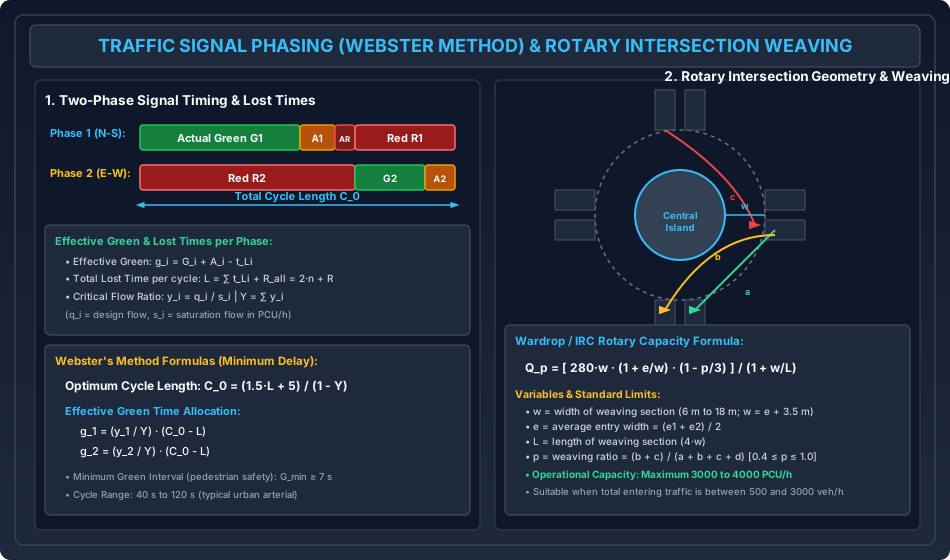
- Effective Green Time (): The usable portion of a phase during which vehicles discharge at the full saturation flow rate: where is actual displayed green, is amber interval, and is total phase lost time.
- Phase Lost Time (): Consists of start-up delay () due to initial driver reaction and acceleration, plus clearance lost time () at the end of the amber interval:
- All-Red Interval (): A clearance period where signals on all approaches show red simultaneously, permitting the last clearing vehicle to exit the conflict box before cross-traffic enters.
6.2 Webster's Method for Optimum Cycle Length
F.V. Webster (1958) utilized extensive computer simulations and empirical observations to formulate the total intersection vehicular delay equation. Minimizing overall delay with respect to cycle length yields Webster's Optimum Cycle Length ():
where:
- = Total lost time per cycle (seconds): (where is number of phases and is total all-red clearance interval).
- = Sum of critical flow ratios: where is the design critical lane flow in phase , and is the corresponding saturation flow.
[!IMPORTANT] Stability Condition: If , demand equals or exceeds saturation flow; cycle length becomes infinite () and the intersection breaks down into permanent oversaturated queuing. For stable operations, design requires .
Effective Green Time Allocation
The total available effective green time across the cycle () is distributed in direct proportion to the critical flow ratios:
Actual displayed green times are obtained as:
6.3 IRC: 93 Signal Design Method
IRC: 93 outlines a practical step-by-step procedure:
- Pedestrian Safety Green Interval (): Mandatory minimum walk time based on pedestrian walking speed :
- Cycle Length Sizing: Check that assigned vehicle green times . Typical cycle times are restricted to .
6.4 The Dilemma Zone Problem
When a driver approaches an intersection at speed and the signal turns amber, they must decide whether to stop or proceed:
- Minimum Stopping Distance ():
- Maximum Distance Traversed during Amber Interval (): where is yellow amber time, is intersection clearance width, and is vehicle length.
- Dilemma Zone: If , a zone exists where the driver can neither stop comfortably before the stop line nor clear the intersection before the red signal appears. To eliminate dilemma zones, the amber interval must satisfy:
7. Intersections & Rotary Design
7.1 At-Grade Intersections
- Unchannelized Intersections: Flared approaches without traffic islands; high accident hazard due to large, uncontrolled conflict areas ( conflict points for a standard 4-leg intersection: crossing, merging, diverging).
- Channelized Intersections: Utilization of directional divisional islands to separate conflicting streams, reduce conflict area, bend conflict angles toward orthogonal (), and establish priority.
7.2 Rotary (Roundabout) Design Mechanics
A rotary intersection is an enlarged channelized at-grade intersection where all converging vehicular traffic streams are converted into a single one-way circulatory movement around a central island.
Geometry of Weaving Sections
- Central Island: Circular or elliptical shape with diameter entry radius.
- Weaving Section: The critical highway zone where merging and diverging traffic streams cross paths along the circulating carriageway.
- Weaving Length (): Distance between entry and exit islands ().
- Weaving Width (): Circulatory carriageway width within the weaving section: where are entry widths, and is average entry width. IRC limits: .
Wardrop's Empirical Rotary Capacity Formula (IRC: 65)
The practical capacity of a rotary weaving section ( in ) is given by Wardrop's equation:
where:
- = width of weaving section in meters ( to )
- = average entry width in meters ()
- = length of weaving section in meters ( ratio between and )
- = Weaving Ratio (Proportion of Weaving Traffic):
where:
- = non-weaving left-turning traffic stream ()
- = weaving traffic stream crossing from left to right ()
- = weaving traffic stream crossing from right to left ()
- = non-weaving outer straight/circulating traffic stream () (IRC mandates: ).
[!TIP] Operational Capacity Threshold: Rotaries operate efficiently when total entering traffic volume is between and . Beyond , rotaries experience severe weaving lock-up, necessitating conversion to grade-separated interchanges.
8. Analytical Derivations
Derivation 1: Theoretical Capacity in Greenshields Model
Starting from Greenshields linear hypothesis:
Using the hydrodynamic identity:
To maximize flow with respect to density :
Dividing by :
Second derivative test for strict concavity:
Substituting into the speed-density relation:
Computing peak capacity :
Derivation 2: Wardrop's Inequality ()
Let a sample of vehicles have individual speeds over a test stretch . By definition:
The variance of speeds with respect to the space mean speed is:
Now, expand in a Taylor series about :
Using binomial expansion :
Summing over all vehicles and dividing by :
Since and :
Dividing both sides by :
Multiplying through by :
Since and , it strictly follows that:
9. Solved Numerical Example 1: Traffic Flow & Speed Modeling
Problem Statement
- The macroscopic traffic behavior on a multi-lane urban arterial conforms to Greenshields model with free-flow speed and jam density .
- (a) Calculate the maximum theoretical flow (capacity ) per lane and the operating speed and density at capacity.
- (b) Determine the traffic speed and flow at density (uncongested) and at density (congested). Compare both flow states.
- A spot speed study measured the instantaneous speeds of five vehicles traversing a trap: .
- (a) Compute the Time Mean Speed () and Space Mean Speed ().
- (b) Calculate the variance about the space mean speed and rigorously verify Wardrop's relation.
Step-by-Step Analytical Solution
Part 1: Greenshields Stream Parameters
-
Capacity and Optimum Parameters:
- Optimum density:
- Optimum speed:
- Theoretical Maximum Flow ():
-
Traffic State 1: Uncongested ():
-
Traffic State 2: Congested / Forced Queue ():
Engineering Insight: Both states exhibit the identical discharge rate (), but State 1 represents safe, fast-moving free flow (), while State 2 represents sluggish, heavily congested queuing ().
Part 2: Speed Means & Wardrop's Verification
Given vehicle spot speeds: , .
-
Time Mean Speed ():
-
Space Mean Speed ():
-
Variance About Space Mean Speed ():
-
Wardrop's Identity Verification:
(Exact identity verified; small difference is higher-order truncated binomial terms in small sample).
10. Solved Numerical Example 2: Signal Design by Webster's Method
Problem Statement
A four-legged urban intersection has two phases:
- Phase 1 (North-South): Design critical approach volume , Saturation flow .
- Phase 2 (East-West): Design critical approach volume , Saturation flow .
- The intersection lost time includes start-up lost time of per phase, amber interval of per phase, and an all-red clearance interval of per cycle. Total cycle lost time .
- Determine the critical flow ratios and overall flow ratio .
- Compute the optimum cycle length () by Webster's method.
- Calculate the available effective green time () and allocate individual effective green times .
- Determine the actual displayed green times .
Step-by-Step Analytical Solution
-
Critical Flow Ratios ():
Stability Check: (Stable, unsaturated flow conditions).
-
Optimum Cycle Length (): Using Webster's formulation with total lost time :
Standard Check: lies within the standard range ().
-
Effective Green Time Allocation: Total available green time in cycle:
- Phase 1 Effective Green:
- Phase 2 Effective Green:
-
Displayed Actual Signal Indications: Taking phase lost time and amber :
- Phase 1 cycle allocation: Green , Amber , All-Red , Red (Total ).
- Phase 2 cycle allocation: Green , Amber , All-Red , Red (Total ).
11. Solved Numerical Example 3: Rotary Roundabout Design
Problem Statement
An urban roundabout is designed with weaving section width , average entry width , and weaving length . The traffic streams traversing the most critical weaving section during peak hour are:
- Non-weaving left-turning stream ():
- Weaving stream crossing from left to right ():
- Weaving stream crossing from right to left ():
- Non-weaving right-turning stream ():
- Check the geometric ratios and against IRC: 65 limits.
- Determine the total volume traversing the weaving section and compute the weaving ratio ().
- Calculate the practical capacity of the rotary () using Wardrop's formula.
- Evaluate the degree of saturation () and determine whether the rotary operates at an acceptable Level of Service.
Step-by-Step Analytical Solution
-
Geometric Proportionality Checks:
- Width-to-Length ratio:
- Entry-to-Weaving width ratio:
-
Traffic Stream Flow & Weaving Proportion ():
- Total entering flow in weaving section:
- Total weaving traffic:
- Weaving Ratio ():
- Check IRC limits: .
-
Rotary Capacity Calculation (): Using Wardrop's equation:
Compute intermediate terms:
- Numerator:
- Denominator:
- Capacity:
-
Degree of Saturation & Level of Service Evaluation:
- Operating Threshold: IRC: 65 specifies that the degree of saturation should not exceed () for design peak flows.
- Conclusion: Since , the rotary operates with ample spare reserve capacity, providing LOS B (Reasonably Free Flow) with minimal queuing delays.
12. Common Misconceptions & Exam Traps
[!WARNING]
1. Time Mean Speed vs. Space Mean Speed in Flow Calculations
- Trap: Calculating flow as .
- Correction: Fundamental traffic flow mechanics strictly require Space Mean Speed: . Time Mean Speed () is always larger (); substituting yields a falsely inflated capacity.
[!WARNING]
2. The Coordinates in Greenshields Model
- Trap: Assuming maximum capacity occurs at free-flow speed or at jam density .
- Correction: Flow is identically zero at both (since ) and (since ). Peak capacity occurs exactly at midpoints:
[!WARNING]
3. Lost Time in Webster's Formula ()
- Trap: Confusing lost time per phase () with total cycle lost time ().
- Correction: In , represents the sum of lost times across all phases in the cycle (). If each phase has lost time in a 2-phase signal, , NOT .
[!WARNING]
4. Weaving Ratio in Roundabout Sizing ()
- Trap: Treating all traffic entering the roundabout as weaving traffic.
- Correction: Left-turning vehicles () and outer circulating vehicles () do not weave; they diverge or merge without crossing paths. Only streams and cross paths. The denominator is the total traffic (), while the numerator is strictly :
13. Quick Revision Summary & Formula Sheet
+---------------------------------------------------------------------------------------------------+
| TRAFFIC ENGINEERING FORMULA SHEET (IRC 93 / IRC 106 / IRC 65)                                     |
+---------------------------------------------------------------------------------------------------+
| 1. Stream Flow Dynamics:                                                                          |
|    - Fundamental Identity:  q = u_s * k                                                           |
|    - Time Headway:          h_t = 3600 / q  (s)                                                   |
|    - Space Headway:         h_s = 1000 / k  (m)                                                   |
|    - Greenshields Model:    u = u_f * (1 - k / k_j)                                               |
|                             Capacity q_max = (u_f * k_j) / 4                                      |
|                             Occurs at u_o = u_f / 2  and  k_o = k_j / 2                           |
|    - Greenberg Model:       u = c * ln(k_j / k)   |   q_max = (c * k_j) / e                       |
|    - Underwood Model:       u = u_f * exp(-k / k_o) |  q_max = (u_f * k_o) / e                    |
+---------------------------------------------------------------------------------------------------+
| 2. Speed Means & Wardrop's Relation:                                                              |
|    - Time Mean Speed (Arithmetic):  u_t = (1 / n) * SUM( u_i )                                    |
|    - Space Mean Speed (Harmonic):   u_s = n / [ SUM( 1 / u_i ) ]                                  |
|    - Wardrop's Fundamental Identity: u_t = u_s + (sigma_s^2 / u_s)   >=  u_s                      |
|    - Percentiles: 98th % (Design), 85th % (Safe Limit), 50th % (Median), 15th % (Minimum)         |
+---------------------------------------------------------------------------------------------------+
| 3. Webster's Signal Timing Method:                                                                |
|    - Optimum Cycle Length:  C_0 = (1.5 * L + 5) / (1 - Y)                                         |
|      * L = Total cycle lost time = SUM( t_Li ) + AR                                               |
|      * Y = Critical flow ratio sum = SUM( y_i ) = SUM( q_i / s_i )  [Stability: Y < 0.85]        |
|    - Effective Green Allocation: g_i = (y_i / Y) * (C_0 - L)                                      |
|    - Actual Displayed Green:     G_i = g_i + t_Li - A_i                                           |
|    - Pedestrian Green Time:      G_ped = 7.0 + W_road / 1.2                                       |
+---------------------------------------------------------------------------------------------------+
| 4. Rotary Roundabout Capacity (Wardrop / IRC: 65):                                                |
|    - Capacity: Q_p = [ 280 * w * (1 + e/w) * (1 - p/3) ] / (1 + w/L)  (PCU/h)                     |
|      * w = Weaving width (6 m to 18 m) = e + 3.5 m                                                |
|      * e = Average entry width = (e1 + e2) / 2                                                    |
|      * L = Weaving length (>= 4 * w)                                                              |
|      * p = Weaving ratio = (b + c) / (a + b + c + d)   [0.40 <= p <= 1.00]                        |
|      * Degree of Saturation: X = V_total / Q_p <= 0.80 (Stable)                                   |
+---------------------------------------------------------------------------------------------------+
14. References & Standard Codes
- Indian Roads Congress (IRC):
- IRC: 106-1990: Guidelines for Capacity of Urban Roads in Plain Areas, New Delhi.
- IRC: 64-1990: Guidelines for Capacity of Roads in Rural Areas, New Delhi.
- IRC: 93-1985: Guidelines on Suitable Design of Traffic Signals, New Delhi.
- IRC: 65-2017: Guidelines for Planning and Design of Roundabouts (First Revision), New Delhi.
- IRC: SP: 41-1994: Guidelines on the Design of At-Grade Intersections, New Delhi.
- National Research Institutions:
- CSIR-CRRI, Indian Highway Capacity Manual (Indo-HCM), Central Road Research Institute, 2017.
- Primary Textbooks:
- Kadiyali, L.R., Traffic Engineering and Transportation Planning, Khanna Publishers, 9th Edition.
- Mannering, F.L. and Washburn, S.S., Principles of Highway Engineering and Traffic Analysis, 7th Edition, Wiley.
- Roess, R.P., Prassas, E.S., and McShane, W.R., Traffic Engineering, 4th Edition, Pearson.