Open Channel Flow Fundamentals: Classification, Velocity Distribution, Resistance Equations & Most Economical Sections
In this chapter (4 topics)
On this page
- 1. Module Overview & Pedagogical Scope
- 2. Official Examination Syllabus Mapping
- 3. Fundamental Physical Principles & Governing Assumptions
- 3.1 The Free Surface & Hydrostatic Pressure Distribution
- 3.2 Velocity Distribution & Isovel Mechanics
- 3.3 Non-Uniform Velocity Correction Coefficients
- 4. Mathematical Derivations & Rigorous Proofs
- Proof 1: Uniform Flow Dynamic Equilibrium & Derivation of Chezy's Formula
- Proof 2: Manning's Resistance Equation & Interrelationships
- Proof 3: Most Economical / Efficient Rectangular Channel Section
- Proof 4: Most Economical / Efficient Trapezoidal Channel Section
- Proof 5: Most Economical Triangular & Circular Sections
- 5. Technical Diagrams & Interactive Architectural Schematics
- Diagram 1: Open Channel Flow Geometry & Velocity Dynamics
- Diagram 2: Most Economical Hydraulic Cross-Sections
- 6. Comparative Engineering Analysis & Parameter Regimes
- Table 6.1: Master Synthesis of Most Economical Channel Geometries
- Table 6.2: Manning Roughness Coefficient n Guidelines (IS 10430: 2000)
- 7. Worked Numerical Examples (Pre-Calculated & Verified)
- Problem 1: Design of Most Economical Trapezoidal Canal
- Problem 2: Velocity Distribution & Kinetic / Momentum Correction Factors
- Problem 3: Partially Full Circular Sewer Hydraulics
- 8. High-Yield Examination Traps & Ambiguities
- Trap 1: The Myth of Maximum Velocity at the Water Surface
- Trap 2: Economical Triangular Section Hydraulic Radius
- Trap 3: Inverting Depths for Maximum Velocity vs Maximum Discharge in Sewers
- Trap 4: Dimensionality of Chezy's C
- 9. Real-World Engineering Applications & Case Studies
- 9.1 The Indira Gandhi Feeder Canal (Rajasthan, India)
- 9.2 Municipal Storm Sewer Design & Self-Cleansing Limits
- 10. Cross-Disciplinary & Downstream Dependencies
- 11. Summary Formula Cheat Sheet & Memory Anchors
- 12. Comprehensive References & Standard Codes
1. Module Overview & Pedagogical Scope
Open channel flow is defined as the flow of liquid (predominantly water) within a conduit or channel possessing a free water surface exposed to the ambient atmosphere. Unlike closed-conduit pressurized pipe flow, where fluid motion is driven by a piezometric pressure gradient (), open channel flow is driven primarily by the component of gravity acting parallel to the channel bed slope.
In civil, environmental, and water resources engineering, open channels encompass natural watercourses (rivers, streams, estuaries) and engineered artificial waterways (irrigation canals, navigation channels, highway drainage ditches, sewers flowing partially full, and aqueducts).
+--------------------------------------------------------------------------------------------------+
|                                    FLOW CLASSIFICATION MATRIX                                    |
+--------------------------------------------------------------------------------------------------+
| Parameter Criterion          | Flow State Classifications & Governing Relations                  |
+------------------------------+-------------------------------------------------------------------+
| Time Dependency              | • Steady Flow:       ∂y/∂t = 0, ∂V/∂t = 0, ∂Q/∂t = 0               |
|                              | • Unsteady Flow:     ∂y/∂t ≠ 0, ∂V/∂t ≠ 0, ∂Q/∂t ≠ 0               |
+------------------------------+-------------------------------------------------------------------+
| Spatial Dependency (Space)   | • Uniform Flow:      ∂y/∂s = 0, ∂V/∂s = 0 (Bed || Surface || HGL)  |
|                              | • Varied / Non-Uniform: ∂y/∂s ≠ 0                                 |
|                              |   - Gradually Varied Flow (GVF): Curvature negligible, dy/dx small|
|                              |   - Rapidly Varied Flow (RVF):   Pronounced curvature, dy/dx large|
|                              |   - Spatially Varied Flow (SVF): Discharge varies along x (dQ/dx≠0)|
+------------------------------+-------------------------------------------------------------------+
| Gravitational Effect         | • Subcritical (Tranquil): Fr < 1.0 (Downstream control, waves run upstream)|
| (Froude Number Fr)           | • Critical State:         Fr = 1.0 (Minimum specific energy)     |
|                              | • Supercritical (Shooting):Fr > 1.0 (Upstream control, waves sweep down)   |
+------------------------------+-------------------------------------------------------------------+
| Viscous Effect               | • Laminar Flow:     Re = (4VR/ν) < 500  (or VR/ν < 500 in open flow)|
| (Reynolds Number Re)         | • Transitional:     500 ≤ Re ≤ 2000                              |
|                              | • Turbulent Flow:   Re > 2000  (Virtually all civil flows)       |
+------------------------------+-------------------------------------------------------------------+
2. Official Examination Syllabus Mapping
Website note: this mapping is from the author’s notes. It has not been checked against the official notification for each examination; confirm the current syllabus with the examining body.
| Examination Body | Primary Syllabus Line | Recurring Problem Archetypes |
|---|---|---|
| GATE CE | Uniform flow, Chezy's and Manning's equations, specific energy, critical depth, most economical sections. | • Analytical proof of best hydraulic dimensions (, half-hexagon ). • Computation of normal depth using iterative Manning equation. • Calculation of Coriolis () and Boussinesq () coefficients from velocity power laws. |
| UPSC ESE | Fluid Mechanics & Hydraulics: Open channel flow, velocity distribution, resistance formulas, efficient cross-sections. | • Multi-variable derivation of trapezoidal section with variable side slope . • Sewer design: Proof of for and for . • Compound channel discharge distribution and equivalent roughness. |
| SSC JE / RRB JE | Hydraulics: Open channels, Chezy and Manning formulas, economical rectangular and trapezoidal sections. | • Direct formula substitutions: , apex angle . • Dimensions of Chezy coefficient (). • Relationship between Chezy , Manning , and Darcy friction factor . |
| State AE / JE | Water Resources & Irrigation Engineering: Channel design and uniform flow. | • Selection of non-scouring and non-silting velocities. • Economical triangular flumes for discharge measurement. |
3. Fundamental Physical Principles & Governing Assumptions
3.1 The Free Surface & Hydrostatic Pressure Distribution
- Atmospheric Datum: The pressure at every point on the free liquid surface is equal to local atmospheric pressure ().
- Hydrostatic Distribution Assumption: In steady uniform flow and gradually varied flow (GVF), where streamlines are straight and parallel, vertical fluid accelerations are zero (). The Navier-Stokes equation along the vertical -axis collapses to the classical hydrostatic law: where is the total water depth and is the vertical elevation measured from the channel bed.
- Streamline Curvature Correction:
- Convex Curvature (Crest of spillway): Centrifugal acceleration acts upwards, opposing gravity. Pressure is sub-hydrostatic ().
- Concave Curvature (Toe of spillway / bucket): Centrifugal acceleration acts downwards, adding to gravity. Pressure is super-hydrostatic ().
3.2 Velocity Distribution & Isovel Mechanics
In an open channel cross-section, velocity is non-uniform due to two distinct physical boundaries:
- Solid Boundary Shear: High viscous and turbulent shear stresses at the solid wetted perimeter retard fluid motion, enforcing the no-slip boundary condition ( at bed and walls).
- Free Surface Air Friction & Secondary Currents: Although air resistance is low, anisotropic turbulent shear stresses drive secondary helical circulations (Prandtl's secondary flow of the second kind). These vortices transport low-momentum fluid from the sidewalls towards the center of the free surface, causing velocity dip:
- The maximum velocity () does not occur at the free water surface, but at a depth of below the surface.
- Mean Velocity Averaging Rules:
- One-Point Method (Shallow Streams, ):
- Two-Point Method (Moderate & Deep Channels, ):
3.3 Non-Uniform Velocity Correction Coefficients
Because velocity varies across the cross-sectional area , the true kinetic energy and momentum fluxes exceed the values computed using the mean velocity :
- Coriolis Coefficient / Kinetic Energy Correction Factor ():
- In uniform prismatic channels: .
- In irregular channels / floodplains: .
- Boussinesq Coefficient / Momentum Correction Factor ():
- In uniform prismatic channels: .
- Theoretical Coupling: For typical logarithmic velocity distributions: (Because , is always strictly greater than or equal to , with . For strictly uniform velocity across the entire area, ).
4. Mathematical Derivations & Rigorous Proofs
Proof 1: Uniform Flow Dynamic Equilibrium & Derivation of Chezy's Formula
Consider a reach of length of an open channel with uniform cross-sectional area , wetted perimeter , and bed slope angle ( for small civil slopes):
                       Free Water Surface (Slope S0)
           --------------------------------------------------
          /                                                 /
         /                     Volume = A * L              /
        /                                                 /
       +-------------------------------------------------+
                          Bed (Slope S0)
-
Equilibrium of Forces along the Flow Direction: In steady uniform flow, acceleration is identically zero (). Therefore, the component of fluid weight driving the flow down the incline must exactly balance the total boundary shear resistance retarding the flow:
-
Weight Component:
-
Boundary Shear Resistance: Assuming a mean boundary shear stress acting over the entire wetted surface area ():
-
Equating Driving and Resisting Forces:
where is the hydraulic radius ().
-
Hydrodynamic Formulation of Boundary Shear: From boundary layer fluid mechanics, boundary shear stress is proportional to dynamic pressure:
where is a dimensionless surface friction coefficient.
-
Solving for Mean Velocity :
Defining the Chezy Discharge Coefficient :
Dimensionality Note: Since has dimensions and has dimensions , the Chezy coefficient is not dimensionless; it possesses the dimensional formula:
Proof 2: Manning's Resistance Equation & Interrelationships
In 1889, Irish engineer Robert Manning empirically unified uniform flow data across diverse channels, proposing:
where is Manning's roughness coefficient ().
Relationship Between Chezy and Manning :
Equating the Chezy and Manning expressions for mean velocity:
Relationship with Darcy-Weisbach Friction Factor :
From the Darcy-Weisbach equation applied to pipe flow of diameter :
For non-circular open conduits, the equivalent hydraulic diameter is . The energy slope :
Equating with Chezy's formula :
Equating with Manning's formula:
Proof 3: Most Economical / Efficient Rectangular Channel Section
A channel section is defined as most economical (or hydraulically most efficient) when it delivers the maximum discharge for a given cross-sectional area , roughness , and bed slope , which by Manning's equation is mathematically identical to minimizing the wetted perimeter for a given area .
-
Geometric Relations for a Rectangular Section: Let bottom width be and depth of flow be .
-
Minimizing Wetted Perimeter with respect to Depth (Constant Area ):
Substitute :
(The bottom width must equal twice the depth of flow!)
-
Check for Minimum (Second Derivative Test):
-
Hydraulic Radius of Economical Rectangular Section:
(The hydraulic radius is exactly half the flow depth!)
-
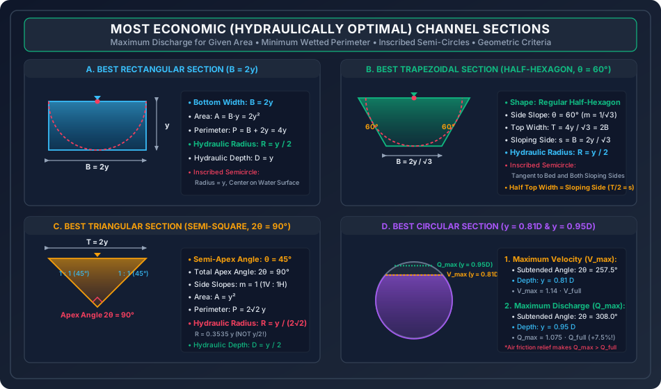
Inscribed Geometric Property: A circle of radius drawn with its center located at the midpoint of the free water surface is exactly tangent to the channel bed and both vertical sidewalls.
Proof 4: Most Economical / Efficient Trapezoidal Channel Section
For a trapezoidal channel with bottom width , depth , and side slopes (slope angle with horizontal ):
       <------------------ Top Width T ------------------>
       \                                                 /
        \                                               /
     s   \                 Depth y                     / s
          \                                           /
           +-----------------------------------------+
             <----------- Bottom Width B ----------->
-
Geometric Parameters:
-
Condition 1: Optimum Proportions for a Given Side Slope : Differentiating with respect to treating and as constants:
Substitute :
Since the top width :
-
Hydraulic Radius of Economical Trapezoidal Section: Substitute into :
-
Condition 2: Optimum Side Slope Angle : To find the best side slope, minimize with respect to treating as constant:
Squaring both sides:
Side slope angle with the horizontal:
-
Geometric Invariance: The Regular Half-Hexagon:
- Sloping side: .
- Top width: .
- Bottom width: .
- Thus: .
- A semi-circle of radius centered at the midpoint of the water surface is simultaneously tangent to the bed and both side slopes.
Proof 5: Most Economical Triangular & Circular Sections
Part A: Triangular Section (V-Flume)
Let the apex half-angle be with side slopes ():
-
Geometric Relations:
-
Minimizing with respect to :
Total Vertex Apex Angle: (A right-angled semi-square triangle!).
-
Hydraulic Radius:
Part B: Circular Conduit (Partially Full Flow)
For a circular channel of diameter with liquid filling up to subtended central angle (in radians):
-
Condition for Maximum Velocity (): By Manning's formula, . Therefore, is maximized when is maximized:
Solving this transcendental equation yields:
-
Condition for Maximum Discharge (): Discharge . Maximizing :
Substituting and : Solving yields:
(Physical insight: At , closing the remaining top adds large wetted perimeter friction along the crown without adding meaningful cross-sectional area, decreasing discharge).
5. Technical Diagrams & Interactive Architectural Schematics
Diagram 1: Open Channel Flow Geometry & Velocity Dynamics
+--------------------------------------------------------------------------------------------------+
| FIGURE 1: OPEN CHANNEL FLOW KINEMATICS, VELOCITY DIP & CORIOLIS / BOUSSINESQ CORRECTIONS         |
+--------------------------------------------------------------------------------------------------+
The schematic below illustrates the fundamental physical contrast between conduit flow under pressure and gravity open channel flow, depicting dynamic shear equilibrium, 2D cross-sectional isovels, the velocity dip phenomenon, and energy/momentum weighting factors.
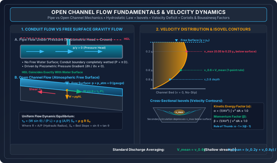
Diagram 2: Most Economical Hydraulic Cross-Sections
+--------------------------------------------------------------------------------------------------+
| FIGURE 2: THE FOUR MOST ECONOMICAL CANAL CROSS-SECTIONS & INSCRIBED CIRCLE GEOMETRY              |
+--------------------------------------------------------------------------------------------------+
The schematic below illustrates the geometric parameters, inscribed semi-circle properties, and critical mathematical thresholds for Rectangular (), Trapezoidal half-hexagon (), Triangular semi-square (), and Circular sewer regimes ( and ).
6. Comparative Engineering Analysis & Parameter Regimes
Table 6.1: Master Synthesis of Most Economical Channel Geometries
| Cross-Section Type | Primary Optimality Criterion | Flow Area | Wetted Perimeter | Hydraulic Radius | Top Width | Hydraulic Depth | Inscribed Circle Tangency |
|---|---|---|---|---|---|---|---|
| Rectangular | Center at water surface; tangent to bed and vertical walls. | ||||||
| Trapezoidal (General ) | Center at water surface; tangent to 3 solid boundaries. | ||||||
| Trapezoidal (Optimum ) | () | Regular half-hexagon; . | |||||
| Triangular | () | Semi-square; (NOT ). | |||||
| Circular () | Occurs at flow depth ; . | ||||||
| Circular () | Occurs at flow depth ; . |
Table 6.2: Manning Roughness Coefficient Guidelines (IS 10430: 2000)
| Channel Boundary Material & Condition | Minimum | Design / Normal | Maximum |
|---|---|---|---|
| Smooth Concrete Lining (Trowel finish) | 0.011 | 0.013 | 0.015 |
| Shotcrete / Gunite Lining | 0.016 | 0.019 | 0.022 |
| Brickwork in Cement Mortar | 0.014 | 0.015 | 0.017 |
| Earthen Channel (Straight, clean, uniform) | 0.018 | 0.022 | 0.025 |
| Earthen Channel with Weeds / Sluggish winding | 0.025 | 0.035 | 0.045 |
| Rubble Riprap / Coarse Gravel Bed | 0.030 | 0.035 | 0.040 |
| Corrugated Metal Pipe (CMP) | 0.021 | 0.024 | 0.027 |
7. Worked Numerical Examples (Pre-Calculated & Verified)
Problem 1: Design of Most Economical Trapezoidal Canal
Problem Statement: An irrigation canal is to be designed as the most economical trapezoidal section to convey a steady discharge . The longitudinal bed slope is (), and the channel is lined with smooth concrete having a Manning roughness coefficient .
- Determine the optimal side slope angle .
- Calculate the required flow depth , bottom width , top width , and flow area .
- Compute the mean velocity of flow and verify that the discharge matches .
Step-by-Step Solution:
-
Optimal Side Slope & Section Shape: For the globally most economical trapezoidal section, the side slope must be a regular half-hexagon:
The geometric parameters in terms of depth are:
-
Manning Discharge Formulation:
Evaluate the constant coefficient:
-
Solving for Depth :
-
Calculating Cross-Sectional Dimensions:
-
Velocity & Discharge Verification:
Check via Manning's formula:
Problem 2: Velocity Distribution & Kinetic / Momentum Correction Factors
Problem Statement: In a wide rectangular river channel of total flow depth , the velocity profile along the vertical centerline follows the 1/6th power law:
where is the height measured upwards from the river bed.
- Determine the depth-averaged mean velocity .
- Compute the Coriolis kinetic energy correction factor .
- Compute the Boussinesq momentum correction factor .
- Check the empirical rule .
Step-by-Step Solution:
-
Mean Velocity Calculation ():
-
Kinetic Energy Correction Factor ():
-
Momentum Correction Factor ():
-
Verification of Rule of Thumb:
Problem 3: Partially Full Circular Sewer Hydraulics
Problem Statement: A concrete circular sewer has internal diameter , bed slope (), and Manning coefficient .
- Compute the velocity and discharge when running completely full under gravity.
- Determine and when the flow depth is ().
- Determine the maximum possible velocity and its corresponding depth.
- Determine the maximum possible discharge and its corresponding depth.
Step-by-Step Solution:
-
Full Flow Parameters ():
-
Partially Full at Depth : The radius is . Water depth is below the center:
Total central angle: .
(Notice that , fulfilling municipal self-cleansing requirements).
-
Condition of Maximum Velocity (): Occurs at , giving flow depth:
At this depth:
-
Condition of Maximum Discharge (): Occurs at , giving flow depth:
At this depth:
(The circular sewer carries MORE discharge at depth than when totally submerged under atmospheric gravity flow!).
8. High-Yield Examination Traps & Ambiguities
[!WARNING]
Trap 1: The Myth of Maximum Velocity at the Water Surface
In textbook ideal 1D flows, students often assume shear stress is zero at the surface, so velocity must be maximum at . In reality, secondary transverse currents and air boundary interaction depress the velocity filament. For competitive exams, remember:
- Maximum velocity occurs at below the surface.
- Mean velocity is measured at below surface (one-point) or average of and below surface (two-point).
- Surface velocity is typically higher than , so .
[!WARNING]
Trap 2: Economical Triangular Section Hydraulic Radius
For rectangular and trapezoidal economical sections, . In haste, students mistakenly write for triangular channels.
- For the most economical triangular section ():
[!WARNING]
Trap 3: Inverting Depths for Maximum Velocity vs Maximum Discharge in Sewers
In GATE and ESE multiple-choice questions, options intentionally invert the depths for circular conduits:
- Maximum Velocity (): Occurs at depth ().
- Maximum Discharge (): Occurs at depth ().
- Mnemonic Anchor: Velocity comes first alphabetically and numerically at lower depth (), while Discharge requires almost the full pipe capacity ().
[!CAUTION]
Trap 4: Dimensionality of Chezy's
Never state that Chezy's is dimensionless. Darcy's is dimensionless, but Chezy's has dimensions:
Manning's has dimensions:
9. Real-World Engineering Applications & Case Studies
9.1 The Indira Gandhi Feeder Canal (Rajasthan, India)
The Indira Gandhi Feeder Canal is one of the largest lined irrigation canals in the world, designed to carry () from Harike Barrage in Punjab to the arid Thar desert in Rajasthan.
- Cross-Section Profile: Designed as an optimal concrete-lined trapezoidal section with side slopes () rather than , because natural soil friction angles cannot sustain a cut without structural earth retaining measures.
- Economic Trade-off: While a half-hexagon () minimizes concrete lining volume, geotechnical slope stability governs in unreinforced earthen excavations, dictating side slopes of to . The hydraulic radius is still maintained as .
9.2 Municipal Storm Sewer Design & Self-Cleansing Limits
In gravity sewer design (CPHEEO Manual on Sewerage and Sewage Treatment):
- Minimum Self-Cleansing Velocity: In order to prevent the deposition of suspended grit, sand, and organic matter, sewers must achieve a minimum velocity of at peak design flow and not less than at minimum daily flow.
- Maximum Non-Scouring Velocity: To prevent erosion and abrasion of the interior pipe invert by rolling pebbles, the maximum velocity is capped at for concrete pipes and for vitrified clay pipes.
- Engineers design sewers to run at to during peak dry weather flow (DWF) to guarantee both adequate self-cleansing velocity and ventilation headspace for toxic hydrogen sulfide () dispersal.
10. Cross-Disciplinary & Downstream Dependencies
                                    +-------------------------------------------------------------+
                                    |                      OCF-01: FUNDAMENTALS                   |
                                    |    Uniform Flow, Chezy, Manning, Economical Cross-Sections   |
                                    +-------------------------------------------------------------+
                                                                   |
                                  +--------------------------------+--------------------------------+
                                  |                                                                 |
                                  v                                                                 v
+-----------------------------------------------------+   +-----------------------------------------------------+
|             OCF-02: CRITICAL FLOW & ENERGY          |   |          IRRI-02: CANAL DESIGN & REGIME             |
|   Specific Energy (E), Froude Number, Bed Transitions|   |   Kennedy & Lacey Silt Theories, Permissible Shear   |
+-----------------------------------------------------+   +-----------------------------------------------------+
                                  |                                                                 |
                                  v                                                                 v
+-----------------------------------------------------+   +-----------------------------------------------------+
|             OCF-03: GRADUALLY VARIED FLOW           |   |       HYDRO-03: STREAM GAUGING & RATING CURVES      |
|   Surface Profiles (M1, M2, S1), Backwater Analysis |   |   Current Meters, Stage-Discharge, Manning Synthesis |
+-----------------------------------------------------+   +-----------------------------------------------------+
- Downstream Module
OCF-02: Uses the normal depth derived here as the baseline for comparing critical depth and classifying channels as mild () or steep (). - Downstream Module
OCF-03: The friction slope in the GVF dynamic equation () is evaluated directly using Manning's equation: . - Irrigation Engineering (
IRRI-02): Directly compares the hydraulic optimal section with Lacey's regime perimeter and Kennedy's non-silting critical velocity .
11. Summary Formula Cheat Sheet & Memory Anchors
| Entity | Primary Formula | Examination Mnemonic / Rule |
|---|---|---|
| Chezy Velocity | "Chezy Sees Roots" () | |
| Manning Velocity | to the power , to the | |
| Chezy vs Manning | Sixth root of divided by | |
| Chezy vs Darcy | Square root of over | |
| Boundary Shear | Mean bed shear balance | |
| Coriolis Factor | Energy | |
| Boussinesq Factor | Momentum ; | |
| Best Rectangle | Bottom width = twice depth | |
| Best Trapezoid | Regular Half-Hexagon: | ; angles |
| Best Triangle | Semi-Square: | Right angle at bottom; |
| Circular | faster than full pipe | |
| Circular | more discharge than full pipe |
12. Comprehensive References & Standard Codes
- Subramanya, K. (2019). Flow in Open Channels, 5th Edition, McGraw-Hill Education, New Delhi.
- Chow, Ven Te (1959). Open-Channel Hydraulics, McGraw-Hill Book Company, New York. (The definitive worldwide treatise on open channel fluid dynamics).
- Henderson, F. M. (1966). Open Channel Flow, Macmillan Publishing, New York.
- Modi, P. N., & Seth, S. M. (2020). Hydraulics and Fluid Mechanics Including Hydraulics Machines, Standard Book House, New Delhi.
- Bureau of Indian Standards (BIS):
- IS 10430: 2000 — Criteria for Design of Lined Canals and Guidelines for Selection of Type of Lining.
- IS 7112: 2002 — Criteria for Design of Cross-Sections for Unlined Canals in Alluvial Soil.
- IS 4713: 1968 — Code of Practice for Installation of Rain Gauges and Channel Gauging Stations.
- Central Public Health and Environmental Engineering Organisation (CPHEEO): Manual on Sewerage and Sewage Treatment Systems, Ministry of Housing and Urban Affairs, Government of India.