Precipitation, Hyetographs, Rain Gauges, Missing Data & Mean Areal Rainfall Estimation
In this chapter (4 topics)
On this page
- 1. Module Scope & Pedagogical Objectives
- 2. Comprehensive Syllabus Mapping
- 3. Physical Principles, Atmospheric Thermodynamics & Flow Regimes
- 3.1 The Catchment Water Budget Equation
- 3.2 Forms of Precipitation
- 3.3 Types of Precipitation (Meteorological Lifting Mechanisms)
- 4. Rigorous Mathematical Formulations & Analytical Derivations
- 4.1 Proof 1: Statistical Adequacy of Rain Gauge Networks
- 4.2 Proof 2: Estimation of Missing Rainfall Data
- 4.3 Proof 3: Consistency of Rainfall Records (Double Mass Curve Analysis)
- 4.4 Proof 4: Catchment Mean Areal Precipitation (barP)
- 4.5 Proof 5: Mathematical Properties of Hyetograph & Mass Curve
- 5. Hand-Coded High-Precision Engineering Visualizations
- 5.1 Diagram 1: Rain Gauge Instruments & Dual Hydro-Meteorological Plots
- 5.2 Diagram 2: Catchment Spatial Averaging (Thiessen vs Isohyetal Methods)
- 6. Comparative Engineering Analysis & Cross-Sectional Synthesis
- 6.1 Rain Gauge Instrumentation Comparison Matrix
- 6.2 Comparison of Catchment Areal Averaging Methods
- 7. Fully Worked Numerical Problems (Pre-Calculated & Verified)
- Problem 1: Statistical Adequacy of Rain Gauge Network
- Problem 2: Missing Data via Normal Ratio & Double Mass Curve Inconsistency
- Problem 3: Mean Areal Rainfall Comparison in a 1200 km2 Catchment
- 8. Critical Exam Traps, Failure Modes & Conceptual Pitfalls
- 9. Real-World Engineering Case Studies & Forensic Failures
- 9.1 The Machchhu Dam II Disaster (Morbi, Gujarat, India, 1979)
- 9.2 Urban Flooding in Chennai (December 2015)
- 10. Cross-Disciplinary & Downstream Dependencies
- 11. High-Yield Revision Formula Cheat Sheet
- 12. Authoritative References & Standards
1. Module Scope & Pedagogical Objectives
Hydrology is the foundational geophysical and civil engineering science that studies the occurrence, circulation, distribution, and properties of water on the Earth and its atmosphere. Engineering Hydrology focuses specifically on quantifying water fluxes to design hydraulic structures (dams, spillways, barrages, culverts, urban drainage networks) and manage regional water resources under conditions of meteorological uncertainty.
At the very head of the hydrologic cycle is Precipitation—the total input of atmospheric moisture condensing and falling under gravity onto a drainage basin. Accurate hydro-meteorological estimation of rainfall depth, spatial distribution, temporal intensity, and station adequacy forms the cornerstone of all downstream hydrologic calculations, including infiltration estimation, hydrograph analysis, flood peak routing, and reservoir sizing.
                                  ATMOSPHERIC MOISTURE (Water Vapor)
                                                ▲
                                                │ Evaporation (E) & Transpiration (T)
                         Precipitation (P)     │
                                │              │
                                ▼              │
               ┌────────────────────────────────────────────────────────────────┐
               │                  DRAINAGE CATCHMENT BASIN                      │
               │                                                                │
               │   Surface Runoff (R) ──► Streams / Rivers ──► Sea / Reservoir  │
               │   Infiltration (F)   ──► Soil Moisture Storage                 │
               │   Percolation (G)    ──► Deep Groundwater Storage (ΔS)         │
               └────────────────────────────────────────────────────────────────┘
The core pedagogical objectives of this module are:
- Formulate the fundamental catchment water budget equation and classify the thermodynamic forms and meteorologic mechanisms of precipitation.
- Examine the operational physics, dimensional standards, and observational protocols of non-recording (Symons gauge) and recording rain gauges (Tipping bucket, Weighing bucket, Natural siphon) conforming to Bureau of Indian Standards (BIS) and World Meteorological Organization (WMO) guidelines.
- Establish the statistical sampling theory governing the adequacy of rain gauge networks and analytically determine the optimum number of stations () to satisfy a prescribed permissible error.
- Derive mathematical methods for interpolating missing rainfall data (Arithmetic Mean vs Normal Ratio Method) and correcting long-term data inconsistencies using Double Mass Curve Analysis.
- Formulate, compare, and apply the three classical methods for computing Catchment Mean Areal Precipitation: the Arithmetic Mean, the Thiessen Polygon (area-weighting), and the Isohyetal (contour integration) methods.
- Analyze the mathematical properties of the Rainfall Hyetograph, the Cumulative Mass Curve of Rainfall, and Depth-Area-Duration (DAD) curves.
2. Comprehensive Syllabus Mapping
This module covers critical syllabus components across all major competitive and professional examinations:
| Examination Body | Specific Syllabus Topics Addressed | Typical Question Pattern |
|---|---|---|
| GATE CE | Hydrologic cycle, precipitation measurement, rain gauge network adequacy, missing data estimation (Normal Ratio), consistency of records (Double Mass Curve), mean areal rainfall (Thiessen and Isohyetal). | 1-mark objective questions on gauge specifications (Symons dimensions, recording types); 2-mark numericals on optimum gauge density (), Thiessen polygon area-weighting, and Normal Ratio missing data. |
| UPSC ESE (Civil) | Hydrologic cycle, water budget equation, precipitation types and forms, rain gauges, adequacy of network, estimation of missing rainfall, double mass analysis, average depth of precipitation over a basin, hyetograph and mass curve. | 10–12 mark conventional derivations of Thiessen/Isohyetal comparisons, network adequacy proofs, and full-scale numerical problems on missing station rainfall and Double Mass slope correction. |
| SSC JE / State AE | Definition of precipitation, Symons gauge rim diameter and height above ground, IS standards for rain gauge density, arithmetic vs Thiessen methods, definition of hyetograph and mass curve. | Direct factual questions on Symons gauge dimensions (127 mm rim, 305 mm height), formula recall for , and qualitative questions on orographic precipitation. |
| RRB JE | Hydrology, rainfall measurement, rain gauges, average rainfall over catchment, rainfall intensity. | Straightforward formula application, unit conversions, definitions of recording vs non-recording gauges. |
3. Physical Principles, Atmospheric Thermodynamics & Flow Regimes
3.1 The Catchment Water Budget Equation
For any natural drainage basin (catchment or watershed) bounded by a topographic ridgeline (the drainage divide), the law of conservation of mass over a specified time interval is expressed as the Hydrologic Continuity Equation:
In depth units (typically mm or cm over the catchment area ):
Where:
- = Precipitation (total atmospheric water input).
- = Surface runoff (direct streamflow exiting the catchment outlet).
- = Net subsurface groundwater outflow leaving the basin boundary.
- = Direct evaporation from surface water bodies, soil, and vegetation canopies.
- = Transpiration by plant vegetative systems (, Evapotranspiration).
- = Total change in hydrologic storage (, where is surface reservoir storage, is unsaturated soil moisture storage, and is saturated groundwater storage).
Annual Water Budget Simplification: Over a long climatic period (e.g., a complete water year of 365 days, or a multi-year average), storage changes cycle through replenishment and depletion such that . Furthermore, in topographically well-defined basins with impermeable bedrock divides, subsurface leakage is negligible (). Hence, the long-term annual water yield simplifies to:
3.2 Forms of Precipitation
Precipitation is defined as any liquid or frozen moisture that condenses out of atmospheric vapor and reaches the earth's surface. In meteorology and civil engineering, it is classified based on particle state and terminal size:
- Rain: Liquid water droplets with diameters strictly greater than (typically ). Droplets larger than become aerodynamically unstable during free fall and rupture into smaller droplets. Rain is further classified by intensity:
- Light rain: Intensity .
- Moderate rain: Intensity .
- Heavy rain: Intensity .
- Drizzle: Minute liquid water droplets with diameters strictly less than , falling so gently that they appear to float in air currents. Rainfall intensity is almost always .
- Snow: Ice crystals aggregated into white, hexagonal, feathery flakes. Fresh uncompacted snow has an average bulk density of approximately (i.e., of fresh snow equals approximately of equivalent liquid water depth).
- Glaze (Freezing Rain): Supercooled liquid raindrops falling through sub-freezing air that freeze instantly upon contact with cold ground, trees, or structures, forming a clear, dense, hazardous ice coating.
- Sleet: Frozen or partially frozen raindrops—clear or translucent ice pellets of diameter , formed when raindrops fall through a deep layer of sub-freezing air near the ground.
- Hail: Irregular spheres or lumps of hard, layered concentric ice with diameters (sometimes reaching or more), formed within violent cumulonimbus convective updrafts.
3.3 Types of Precipitation (Meteorological Lifting Mechanisms)
Precipitation cannot occur without dynamic vertical lifting of moist air, which induces adiabatic cooling, condensation at the dew point temperature, droplet coalescence, and gravitational precipitation. Based on the mechanism driving vertical ascent:
- Convective Precipitation:
- Caused by intense localized solar heating of the earth's ground surface. The heated air expands, becomes buoyant, and rises rapidly in strong vertical updrafts ().
- Characterized by: High intensity, short duration, localized areal coverage (often ), accompanied by thunder, lightning, and microbursts (e.g., tropical summer afternoon thunderstorms).
- Orographic Precipitation:
- Occurs when moist air masses are mechanically forced upward by topographic barriers such as mountain ridges (e.g., the Western Ghats or Himalayas in India).
- As the air ascends the windward slope, it expands adiabatically, cools, and unloads immense precipitation (e.g., Cherrapunji / Mawsynram, Mahabaleshwar).
- Descending the leeward slope, the air compresses, warms adiabatically, and its relative humidity drops, creating a dry, arid rain shadow region (e.g., the Deccan Plateau east of the Western Ghats).
- Cyclonic (Frontal) Precipitation:
- Generated by large-scale atmospheric pressure depressions. In temperate zones, a warm front (warm moist air gliding smoothly over a retreating cold wedge) produces steady, widespread, light-to-moderate rain over thousands of square kilometers. A cold front (dense cold wedge undercutting warm moist air) produces narrow, intense squall lines.
- In tropical regions, non-frontal tropical cyclones (depressions in the Bay of Bengal and Arabian Sea) produce devastatingly heavy rainfall over coastal catchments.
4. Rigorous Mathematical Formulations & Analytical Derivations
4.1 Proof 1: Statistical Adequacy of Rain Gauge Networks
In any catchment of area , rainfall is sampled at a finite number () of discrete point rain gauge stations. Because precipitation exhibits high spatial variability, the arithmetic mean of these stations () is only a statistical sample estimate of the true catchment average ().
To ensure that the estimated mean areal rainfall has an allowable percentage error not exceeding at a specified statistical confidence level, we apply sampling theory.
Let the annual rainfall at existing stations be . The sample mean is:
The sample standard deviation is:
The dimensionless Coefficient of Variation (), which measures the relative spatial dispersion of rainfall across the basin:
According to the Central Limit Theorem of statistics, the standard error of the sample mean () for a network of stations is:
The allowable relative error (expressed as a percentage of the mean ) is defined as:
Squaring both sides and solving for the Optimum Number of Stations ():
Where:
- = Optimum number of rain gauge stations required in the catchment.
- = Coefficient of variation of rainfall across the existing stations ().
- = Permissible percentage error in the estimation of the catchment mean precipitation (typically specified as to ).
Engineering Decision Rules:
- If : The existing network of stations is adequate to satisfy the allowable error limit . No additional stations are needed.
- If : The existing network is inadequate. The minimum additional number of stations required is:
BIS / WMO Recommended Network Density Standards (IS 4987: 1994):
- Flat plains of temperate, Mediterranean, and tropical zones: 1 station per .
- Mountainous regions of temperate, Mediterranean, and tropical zones: 1 station per .
- Arid and polar zones: 1 station per .
- Mandatory Recording Gauge Fraction: At least of the total stations in the network must be equipped with self-recording instruments.
4.2 Proof 2: Estimation of Missing Rainfall Data
Occasionally, a rain gauge station (say station ) fails to record rainfall during a storm due to instrument malfunction, absence of the observer, or physical vandalism. To reconstruct the continuous meteorological series, the missing value is estimated using data from surrounding index stations () whose normal annual precipitations are known.
Let:
- = Missing storm precipitation at station .
- = Normal annual precipitation at station (based on the standard 30-year climatological average).
- = Recorded storm precipitations at nearby index stations.
- = Normal annual precipitations at the index stations.
Method 1: Simple Arithmetic Mean Method
Applicability Criterion: If the normal annual precipitation at each index station differs by less than from that of station :
Under this condition of regional climatological homogeneity, the storm rainfall at is simply the arithmetic average of the surrounding stations:
Method 2: Normal Ratio Method
Applicability Criterion: If the normal annual precipitation at any index station differs by more than from :
In this case, simple arithmetic averaging introduces severe bias. The precipitation at each index station must be weighted in direct proportion to the ratio of normal annual rainfalls:
Multiplying both sides by yields the celebrated Normal Ratio Equation:
Method 3: Inverse Distance Weighting Method (US National Weather Service)
When normal annual precipitations are unavailable, point estimates can be derived from geographic coordinates using the distance between index station and station :
4.3 Proof 3: Consistency of Rainfall Records (Double Mass Curve Analysis)
A rain gauge record is termed consistent if the recorded values represent true variations in climatic events, free from artificial local trends. In practice, long-term records (spanning decades) frequently become inconsistent due to:
- Relocation of the rain gauge station to a new site (even a shift of a few hundred meters or a change in elevation).
- Change in the physical exposure of the gauge (e.g., growth of surrounding trees or erection of new buildings).
- Replacement of the instrument type or change in the observer's reading technique.
To detect and adjust for such inconsistencies, the Double Mass Curve technique is applied.
                    Double Mass Curve Analysis

   Accumulated Precipitation at Station X (Σ Px)
        │
        │                                 / Slope = Sc (Recent reliable period)
        │                                /
        │                      Break ───•
        │                              /
        │                             /  Slope = Sa (Older period requiring correction)
        │                            /
        │                           /
        └──────────────────────────/──────────────────────────►
            Accumulated Average of Index Stations (Σ P_avg)
Analytical Procedure:
- Select a group of 5 to 10 reliable, permanent index stations surrounding the suspicious station .
- Arrange annual precipitation records in reverse chronological order (most recent year at the top, oldest year at the bottom).
- Compute the annual average precipitation of the index stations for each year: .
- Compute the cumulative rainfall for station () and for the index group ().
- Plot on the vertical -axis against on the horizontal -axis.
- Interpretation of Slope:
- If the station record is consistent, the points lie along a single straight line.
- If a change in the physical regime occurred in year , a distinct break in slope appears at that point.
- Correction of Inconsistent Past Records: The recent slope represents current reliable conditions. All historic records prior to the break (which followed slope ) must be corrected by multiplying by the slope ratio:
Where:
- = Corrected annual precipitation for any year prior to the break.
- = Originally recorded annual precipitation.
- = Corrected slope of the double mass curve (recent period).
- = Original slope of the curve during the period when the record was taken.
4.4 Proof 4: Catchment Mean Areal Precipitation ()
A rain gauge measures rainfall depth at a single point (). For catchment hydrologic models, the total volume of water falling over the entire watershed area must be quantified as a spatially averaged uniform depth :
Because is known only at discrete gauge points, three spatial integration techniques are used:
1. Arithmetic Mean Method
The simplest method, computed as the unweighted mean of all stations situated strictly inside the catchment:
Limitations: Valid ONLY if the catchment is flat, the rain gauges are uniformly spaced, and individual station readings deviate minimally from the mean. Outside stations are ignored entirely.
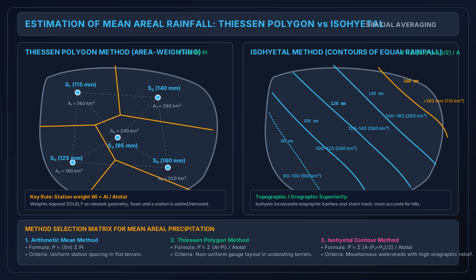
2. Thiessen Polygon Method (Area-Weighting)
Devised by A. H. Thiessen (1911), this method assigns a polygonal tributary influence area to each rain gauge station based on spatial proximity.
Geometric Construction Algorithm:
- Connect adjacent rain gauge stations with straight dashed lines, forming a network of non-overlapping triangles (Delaunay triangulation).
- Construct the perpendicular bisector of each connecting line.
- The intersections of these perpendicular bisectors form closed convex polygons around each station.
- Truncate the outer boundaries of the polygons at the physical watershed divide.
- Planimeter the enclosed polygon area corresponding to station .
The mean areal precipitation is the area-weighted average:
Defining the dimensionless Thiessen Station Weight ():
Critical Engineering Properties:
- Stations located outside the catchment boundary can have polygons that overlap the basin interior, meaning outside stations are rigorously included with weight .
- The weights depend solely on the geometric coordinates of the stations, NOT on rainfall depths. Hence, for a fixed network, the weights are calculated once and applied to all storms.
- If a new station is added or an existing station is relocated, the entire network of polygons must be reconstructed.
3. Isohyetal Method (Contour Integration)
An isohyet is a contour line joining points of equal rainfall depth across a geographical region.
Analytical Formulation:
- Plot recorded station rainfalls on a topographic base map.
- Interpolate lines of equal rainfall (isohyets) at uniform contour intervals (e.g., ), taking into account known orographic features, mountain ridges, and storm tracks.
- Measure the net area enclosed between two consecutive isohyets and , denoted as .
- The average rainfall over this inter-isohyetal strip is taken as the arithmetic mean:
- The total volumetric water input is:
- The catchment mean areal precipitation is:
Superiority: The Isohyetal Method is universally acknowledged as the most accurate method in mountainous terrain because an experienced hydrologist can warp the isohyets to account for windward orographic enhancement and leeward rain shadows.
4.5 Proof 5: Mathematical Properties of Hyetograph & Mass Curve
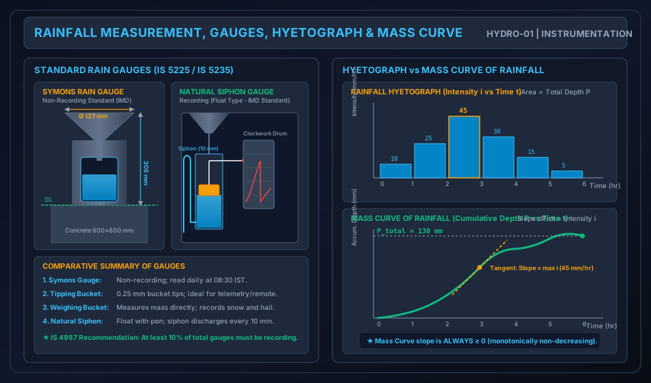
1. The Rainfall Hyetograph:
A plot of rainfall intensity (, mm/hr) on the vertical axis against time (, hr) on the horizontal axis, typically displayed as a discrete step-bar chart.
- The area under the hyetograph between time and represents the total rainfall depth accumulated during that interval:
- For discrete time intervals :
2. The Mass Curve of Rainfall:
A plot of cumulative accumulated precipitation () versus elapsed time (), recorded continuously by recording rain gauges.
- Mathematical relation:
- The instantaneous rainfall intensity at any moment is the first derivative (slope) of the mass curve:
- Fundamental Mathematical Rule: Since precipitation depth cannot physically decrease over time, at all times. Hence, the Mass Curve of Rainfall is a monotonically non-decreasing function. Periods of zero slope () indicate dry cessations of rainfall.
3. Depth-Area-Duration (DAD) Relationships:
For a storm of given duration , the maximum average precipitation depth decreases progressively as the catchment area increases. This phenomenon is modeled by the empirical Horton-type exponential decay formula:
Where is the maximum point rainfall at the storm eye, and and are regional constants.
5. Hand-Coded High-Precision Engineering Visualizations
5.1 Diagram 1: Rain Gauge Instruments & Dual Hydro-Meteorological Plots
The following hand-coded SVG illustrates the internal cross-sectional architecture of standard rain gauges (Symons non-recording gauge and Natural Siphon float recording gauge) alongside the paired plots of the Rainfall Hyetograph and Cumulative Mass Curve.
5.2 Diagram 2: Catchment Spatial Averaging (Thiessen vs Isohyetal Methods)
The following hand-coded SVG details the geometric construction of Thiessen polygons (perpendicular bisectors and tributary areas) and compares it with the contour integration of Isohyetal bands over an identical watershed.
6. Comparative Engineering Analysis & Cross-Sectional Synthesis
6.1 Rain Gauge Instrumentation Comparison Matrix
| Parameter / Feature | Symons Rain Gauge | Tipping Bucket Gauge | Weighing Bucket Gauge | Natural Siphon (Float) Gauge |
|---|---|---|---|---|
| Category | Non-recording | Recording (Digital pulses) | Recording (Analog / Digital) | Recording (Analog chart) |
| Collector Rim Diameter | () | () | ||
| Height of Rim above GL | () | |||
| Operating Mechanism | Funnel discharges into glass bottle; read manually. | Two balanced buckets pivot on knife edge; tips every . | Spring scale records gross weight of bucket + water. | Float moves vertical pen rod on rotating clockwork drum. |
| Siphoning / Reset | None (manual emptying). | Continuous self-emptying per tip. | Must be periodically emptied manually. | Built-in siphon automatically discharges every . |
| Snow / Hail Capability | No (funnel chokes; requires snow tube). | Poor (freezes without internal heater). | Excellent (measures snow, hail, rain mass directly). | No (cannot measure solid snow). |
| Telemetry Suitability | Impossible (requires human observer). | Ideal for automatic weather stations (AWS). | Good with electronic load cells. | Low (traditional mechanical chart). |
| Primary Standard | IS 5225: 1992 (IMD Standard). | WMO No. 8 Guidelines. | US National Weather Service. | IS 5235: 1992 (IMD Standard). |
6.2 Comparison of Catchment Areal Averaging Methods
| Attribute | Arithmetic Mean Method | Thiessen Polygon Method | Isohyetal Contour Method |
|---|---|---|---|
| Mathematical Basis | Simple average: . | Area-weighting: . | Contour integration: . |
| Topographic Relief Handling | Completely ignores topography and relief. | Accounts for spatial layout, but assumes linear gradient between stations. | Accurately accounts for orographic barriers and storm tracks. |
| Outside Station Usage | Excluded completely. | Included if polygon boundary enters basin. | Included during contour interpolation. |
| Weight Flexibility | Equal weight () to all stations. | Fixed geometric weights (). | Variable weights per storm event. |
| Re-calculation Overhead | Instantaneous. | Polygons fixed until station added/removed. | Isohyets must be redrawn for every single storm. |
| Best Applicable Domain | Flat terrain with dense uniform network. | Undulating terrain with non-uniform gauges. | Mountainous catchments with high orographic relief. |
7. Fully Worked Numerical Problems (Pre-Calculated & Verified)
Problem 1: Statistical Adequacy of Rain Gauge Network
Statement: A river drainage catchment has an area of and currently contains operational rain gauge stations. The recorded annual precipitation values at these six stations are:
- Calculate the mean annual precipitation and the sample standard deviation .
- Determine the coefficient of variation () of the rainfall across the catchment.
- If the permissible percentage error in the estimation of the catchment mean annual precipitation is , determine whether the existing network is adequate. How many additional stations are needed?
- If water resource authorities tighten the allowable error to , compute the revised optimum number of stations () and determine the additional stations required.
Step-by-Step Solution:
Step 1: Mean Annual Precipitation ()
Step 2: Sample Standard Deviation ()
Compute the squared deviations :
Sample variance:
Sample standard deviation:
Step 3: Coefficient of Variation ()
Step 4: Network Adequacy for
Since , the existing network of 6 stations is fully adequate to estimate the catchment mean rainfall within an error margin.
Step 5: Revised Network Adequacy for
Under a strict error threshold, the optimum number of stations is .
Problem 2: Missing Data via Normal Ratio & Double Mass Curve Inconsistency
Statement: Part A (Missing Rainfall): A drainage basin contains four rain gauge stations: , and . During a severe storm, station failed to record precipitation. The recorded storm precipitation and long-term normal annual precipitation for all stations are:
- Station : Storm , Normal
- Station : Storm , Normal
- Station : Storm , Normal
- Station : Storm , Normal
Test whether the Simple Arithmetic Mean is applicable or if the Normal Ratio Method must be enforced. Compute the missing storm rainfall .
Part B (Double Mass Curve Correction): The rain gauge at Station was relocated to a new elevated site in the year 2010. A double mass curve plotted between cumulative annual rainfall at and the cumulative average of 10 surrounding base stations reveals a clear break in slope in 2010.
- Slope after 2010 (current, reliable period ): .
- Slope before 2010 (original period requiring adjustment ): .
- The historical annual rainfall recorded at Station in the year 2005 was .
Calculate the corrected annual precipitation for Station for the year 2005.
Step-by-Step Solution:
Part A: Testing Applicability & Estimating
Check the percentage deviation of normal annual precipitation at index stations from station :
Evaluating deviations:
- Station :
- Station :
- Station :
Since stations () and () deviate by more than , the Simple Arithmetic Mean Method is invalid. The Normal Ratio Method must be used.
Applying the Normal Ratio Equation with :
Compute each normalized component:
(Note: Simple arithmetic mean would have given , introducing a severe error).
Part B: Double Mass Curve Slope Correction
The correction ratio to be applied to all pre-2010 records is:
The corrected annual rainfall at Station in 2005 is:
Problem 3: Mean Areal Rainfall Comparison in a Catchment
Statement: A catchment has a total area of .
-
Thiessen Polygon Analysis: Five rain gauge stations inside and near the basin recorded the following precipitation depths, with their respective Thiessen polygon areas measured as:
- Station 1: , Area
- Station 2: , Area
- Station 3: , Area
- Station 4: , Area
- Station 5: , Area
Compute the Thiessen weights , the mean areal rainfall , and compare it with the simple Arithmetic Mean .
-
Isohyetal Analysis: An isohyetal map constructed for the same storm event yielded the following inter-isohyetal zones and planimetered areas:
- Isohyet : Area , average depth
- Between and : Area
- Between and : Area
- Between and : Area
- Between and : Area
Determine the total volumetric precipitation input over the catchment in cubic meters () and the mean areal rainfall . Compute the percentage difference between the Thiessen and Isohyetal estimates.
Step-by-Step Solution:
Part 1: Thiessen Polygon Computation
Verify total area:
Compute station weights :
- Sum of weights:
Compute weighted contributions :
- Station 1:
- Station 2:
- Station 3:
- Station 4:
- Station 5:
Simple Arithmetic Mean:
(Notice that the Arithmetic Mean underestimates the true spatial storm input by because it gives equal weight to Station 3 () which has a small area, while under-weighting Station 4 () which controls over of the watershed).
Part 2: Isohyetal Method Computation
Verify total area:
Compute the average rainfall and product for each zone:
- Zone :
- Zone :
- Zone :
- Zone :
- Zone :
Sum of volumetric products:
Mean Areal Rainfall:
Total Precipitation Volume ():
Percentage Difference:
8. Critical Exam Traps, Failure Modes & Conceptual Pitfalls
   ┌───────────────────────────────────────────────┬───────────────────────────────────────────────┐
   │             EXAM TRAP / MISCONCEPTION         │            RIGOROUS SCIENTIFIC REALITY        │
   ├───────────────────────────────────────────────┼───────────────────────────────────────────────┤
   │ 1. Dividing by m instead of (m - 1) when      │ In network adequacy N = (Cv/ε)², sample       │
   │    calculating standard deviation σ.          │ variance MUST use Bessel's correction (m - 1) │
   │                                               │ because m is small (typically 5 to 10).       │
   ├───────────────────────────────────────────────┼───────────────────────────────────────────────┤
   │ 2. Always using Arithmetic Mean for missing   │ Check if |Ni - Nx|/Nx exceeds 10% for ANY     │
   │    station rainfall.                          │ single station! If even one station exceeds   │
   │                                               │ 10%, you MUST use Normal Ratio Method.        │
   ├───────────────────────────────────────────────┼───────────────────────────────────────────────┤
   │ 3. Inverting the Double Mass correction ratio │ Correction factor is Sc / Sa (Recent Correct  │
   │    as Sa / Sc instead of Sc / Sa.             │ Slope / Old Biased Slope). Pre-break values   │
   │                                               │ are multiplied by (Sc / Sa).                  │
   ├───────────────────────────────────────────────┼───────────────────────────────────────────────┤
   │ 4. Assuming Thiessen weights change with      │ Thiessen weights Wi = Ai / Atotal depend ONLY │
   │    every storm event.                         │ on gauge coordinates/geometry! They remain   │
   │                                               │ constant for all storms until network changes.│
   ├───────────────────────────────────────────────┼───────────────────────────────────────────────┤
   │ 5. Discarding stations located outside the    │ Out-of-basin stations CAN have Thiessen       │
   │    catchment divide in Thiessen method.       │ polygons that cross into the basin. They MUST │
   │                                               │ be included with their enclosed area Ai.      │
   ├───────────────────────────────────────────────┼───────────────────────────────────────────────┤
   │ 6. Believing a Mass Curve of Rainfall can     │ Cumulative rainfall CANNOT decrease. Slope    │
   │    have a negative slope.                     │ dP/dt ≥ 0 always. It is strictly monotonic.   │
   └───────────────────────────────────────────────┴───────────────────────────────────────────────┘
9. Real-World Engineering Case Studies & Forensic Failures
9.1 The Machchhu Dam II Disaster (Morbi, Gujarat, India, 1979)
- Background: In August 1979, the Machchhu Dam II collapsed following an unprecedented catastrophic storm, causing thousands of casualties in the downstream city of Morbi.
- Hydro-Meteorological Cause: The original spillway was designed for a peak design flood of , derived from short-term rain gauge records that severely underestimated maximum possible precipitation. An extraordinary cyclonic cloudburst dumped over of rain in 24 hours across the upstream catchment, generating a peak inflow of over (nearly three times spillway capacity), overtopping and washing out the earthen embankments.
- Engineering Lesson: Rain gauge network adequacy, historical record consistency (Double Mass checks), and rigorous depth-area-duration (DAD) analysis are vital to ensure design flood estimations withstand rare multi-century hydrologic extremes.
9.2 Urban Flooding in Chennai (December 2015)
- Background: In December 2015, extreme cyclonic depression rainfall dumped over of rain in 24 hours over the Adyar and Cooum river catchments, completely inundating Chennai.
- Forensic Finding: A major post-disaster analysis revealed that existing non-recording rain gauges could only provide 24-hour accumulated depths, masking short-term extreme burst intensities () that overwhelmed urban drainage.
- Remediation: The India Meteorological Department (IMD) and state authorities subsequently overhauled the basin with real-time telemetry-equipped tipping-bucket automatic weather stations (AWS) to produce continuous 15-minute hyetographs for automated flood warning systems.
10. Cross-Disciplinary & Downstream Dependencies
                              ┌──────────────────────────────────────────────┐
                              │  HYDRO-01: Precipitation & Mean Areal Rain   │
                              │            (Rain Gauges, Thiessen, Hyetograph)│
                              └──────────────────────┬───────────────────────┘
                                                     │
                                                     ▼
                              ┌──────────────────────────────────────────────┐
                              │ HYDRO-02: Abstractions from Precipitation    │
                              │           (Evaporation, Infiltration, φ-Index│
                              └──────────────────────┬───────────────────────┘
                                                     │ Effective Rainfall Hyetograph (ERH)
                                                     ▼
                              ┌──────────────────────────────────────────────┐
                              │ HYDRO-03: Streamflow Hydrographs & Unit      │
                              │           Hydrograph Convolution Theory       │
                              └──────────────────────┬───────────────────────┘
                                                     │ Peak Flood Discharge (Q_p)
                                                     ▼
                              ┌──────────────────────────────────────────────┐
                              │ IRRI-03: Spillway Design Capacity &          │
                              │          Dam Crest Freeboard Determination   │
                              └──────────────────────────────────────────────┘
- Direct Downstream Prerequisites:
HYDRO-02: Infiltration indices (-index and -index) require the gross rainfall hyetograph to subtract abstraction losses and deduce the Effective Rainfall Hyetograph (ERH).HYDRO-03: Unit Hydrograph theory convolving the ERH to generate the Direct Runoff Hydrograph (DRH).HYDRO-04: Flood frequency analysis and Gumbel extreme value distribution.IRRI-02/IRRI-03: Catchment yield calculations for canal headworks and spillway sizing.
11. High-Yield Revision Formula Cheat Sheet
12. Authoritative References & Standards
- Subramanya, K. Engineering Hydrology. 5th ed., McGraw Hill Education (India), 2021. (The standard authoritative reference for Indian university and competitive examinations).
- Chow, Ven Te, Maidment, D. R., and Mays, L. W. Applied Hydrology. McGraw-Hill Book Company, New York, 1988. (The classic international textbook on mathematical hydrologic principles).
- Linsley, R. K., Kohler, M. A., and Paulhus, J. L. H. Hydrology for Engineers. McGraw-Hill, New York, 1982.
- Bureau of Indian Standards (BIS):
- IS 4987: 1994 (Reaffirmed 2019): Recommendations for Installation and Design of Rain Gauge Networks.
- IS 5225: 1992 (Reaffirmed 2018): Specification for Rain Gauge, Non-Recording (Symons Type).
- IS 5235: 1992 (Reaffirmed 2018): Specification for Rain Gauge, Natural Siphon Type (Recording).
- World Meteorological Organization (WMO):
- WMO No. 168: Guide to Hydrological Practices: Volume I - Hydrology: From Measurement to Hydrological Information. 6th ed., Geneva, Switzerland, 2008.
- WMO No. 8: Guide to Meteorological Instruments and Methods of Observation.
- Reddi, P. Jaya Rami. A Text Book of Hydrology. Laxmi Publications, New Delhi, 2011.