Streamflow Measurement, Hydrograph Components, Baseflow Separation, Unit Hydrograph Theory & S-Curve Method
In this chapter (4 topics)
On this page
- 1. Module Scope & Pedagogical Objectives
- 2. Comprehensive Syllabus Mapping
- 3. Physical Principles, Hydrograph Mechanics & Streamflow Hydraulics
- 3.1 Streamflow Gauging Hydraulics
- 3.2 Stage-Discharge Rating Curves & Loop Hysteresis
- 3.3 Anatomy of a Flood Hydrograph
- 3.4 Baseflow Separation Techniques
- 4. Rigorous Mathematical Formulations & Analytical Derivations
- 4.1 Proof 1: The Area-Velocity Mid-Section Method
- 4.2 Proof 2: Direct Runoff Volume & Unit Hydrograph Scaling
- 4.3 Proof 3: The S-Curve (Summation Curve) Method
- 5. Hand-Coded High-Precision Engineering Visualizations
- 5.1 Diagram 1: Streamflow Gauging, Current Meters & Rating Curve Loop Hysteresis
- 5.2 Diagram 2: Flood Hydrograph Anatomy, Baseflow & S-Curve Duration Conversion
- 6. Comparative Engineering Analysis & Cross-Sectional Synthesis
- 6.1 Streamflow Velocity Measurement Methods Comparison
- 6.2 Unit Hydrograph Duration Conversion: Superposition vs S-Curve
- 7. Fully Worked Numerical Problems (Pre-Calculated & Verified)
- Problem 1: Current Meter River Gauging & Stage-Discharge Rating Curve
- Problem 2: Derivation of 4-hr Unit Hydrograph from a Storm Hydrograph
- Problem 3: Unit Hydrograph Duration Conversion via S-Curve (4-hr to 8-hr UH)
- 8. Critical Exam Traps, Failure Modes & Conceptual Pitfalls
- 9. Real-World Engineering Case Studies & Forensic Failures
- 9.1 The Austin Dam Failure (Pennsylvania, USA, 1911)
- 9.2 Kerala Floods Hydrograph Inflow Miscalculation (August 2018)
- 10. Cross-Disciplinary & Downstream Dependencies
- 11. High-Yield Revision Formula Cheat Sheet
- 12. Authoritative References & Standards
1. Module Scope & Pedagogical Objectives
Streamflow—the discharge of water flowing in a natural river channel—is the only phase of the hydrologic cycle that is integrated over the entire catchment area and can be measured directly with high volumetric precision. While precipitation and infiltration occur as distributed spatial fields across thousands of hectares, the stream network gathers this flux and funnels it through a single topographic outlet: the stream gauging station.
The hydrograph—a continuous time-series record of stream discharge ( vs )—embodies the dynamic response of a drainage basin to storm events. In 1932, Leroy K. Sherman formulated the Unit Hydrograph (UH) Theory, which stands as one of the most brilliant and enduring conceptual breakthroughs in engineering hydrology. By treating the drainage basin as a linear, time-invariant black-box system, Unit Hydrograph theory enables hydrologists to predict the peak flood discharge, time to peak, and complete direct runoff hydrograph for any anticipated rainstorm design event.
   Excess Rainfall Hyetograph (ERH)          Drainage Catchment Basin (Transfer Function)          Direct Runoff Hydrograph (DRH)
   ┌───────────────────────────────┐                  ┌────────────────────────┐                  ┌───────────────────────────────┐
   │ P_eff Depth = 1.0 cm          │ ───────────────► │ Linear System Operator │ ───────────────► │ Q_DRH(t) = R × U(t)           │
   │ Storm Duration = D hours      │                  │ Sherman UH: U_D(t)     │                  │ Volume = 10,000 × A × R  (m³) │
   └───────────────────────────────┘                  └────────────────────────┘                  └───────────────────────────────┘
The core pedagogical objectives of this module are:
- Examine the mechanical principles, instrumentation, and observational protocols of Streamflow Measurement, focusing on stage gauges, current meter velocity sampling ( and ), and the Area-Velocity mid-section integration method.
- Formulate the mathematical structure of the Stage-Discharge Rating Curve (), evaluate shifting controls, and analyze unsteady flood wave loop rating curve hysteresis via the Jones formula.
- Deconstruct the physical anatomy of the Flood Hydrograph (rising limb, crest segment, and recession limb) and compare classical Baseflow Separation Techniques to isolate the Direct Runoff Hydrograph (DRH).
- Establish the fundamental postulates (Linear Proportionality and Time Invariance) and catchment domain boundaries of Sherman's Unit Hydrograph Theory.
- Derive Unit Hydrographs from isolated single-peaked storm hydrographs, and verify the unit depth conservation property ( of direct runoff).
- Formulate and apply the Method of Superposition (for integer multiples ) and the S-Curve (Summation Curve) Method for converting Unit Hydrographs to arbitrary storm durations ().
2. Comprehensive Syllabus Mapping
This module addresses primary syllabus components across all national civil engineering examinations:
| Examination Body | Specific Syllabus Topics Addressed | Typical Question Pattern |
|---|---|---|
| GATE CE | Streamflow measurement, stage-discharge relation, rating curves, hydrograph analysis, baseflow separation, unit hydrograph theory, S-curve derivation, changing unit hydrograph duration. | 1-mark questions on current meter sampling depths () and UH assumptions; 2-mark numericals on rating curve parameter fitting, deriving DRH from complex storms, and S-curve tabular conversions. |
| UPSC ESE (Civil) | Measurement of streamflow, current meters, stage-discharge curves, flood hydrographs, components, baseflow separation methods, unit hydrograph, derivation of unit hydrographs, S-curve method, synthetic unit hydrographs. | 12–20 mark conventional questions on complete tabular derivation of -hr UH, baseflow separation by straight line/two-line methods, and converting 4-hr UH to 6-hr or 8-hr UH via S-curve. |
| SSC JE / State AE | Methods of measuring stream velocity, current meter formula , definition of unit hydrograph, unit storm duration, baseflow separation, S-curve equilibrium discharge . | Direct formula recall (), velocity depth questions ( for shallow vs and for deep streams), and single-step UH scaling calculations. |
| RRB JE | Measurement of river discharge, hydrograph, unit hydrograph, peak runoff, flood discharge. | Conceptual questions on hydrograph components, linearity assumptions, and unit hydrograph definitions. |
3. Physical Principles, Hydrograph Mechanics & Streamflow Hydraulics
3.1 Streamflow Gauging Hydraulics
Streamflow (, ) cannot be measured directly in a natural river without continuous physical measurement of two fundamental state variables: Stage () and Mean Flow Velocity ().
1. Stage Measurement:
The stage (gauge height, ) is the elevation of the water surface above an established reference datum.
- Non-Recording Gauges: Sectional vertical staff gauges painted with millimeter graduations, or wire-weight gauges suspended from bridge piers.
- Recording Gauges: Float-operated autographic chart recorders operating inside a stilling well connected to the river through intake pipes; or pneumatic bubble gauges (gas-purge pressure systems) that measure the hydrostatic pressure required to force nitrogen gas bubbles out of an orifice anchored at the river bed.
2. Velocity Measurement & Current Meters:
River flow is turbulent with complex boundary-layer shear. Point velocity is measured using calibrated Current Meters:
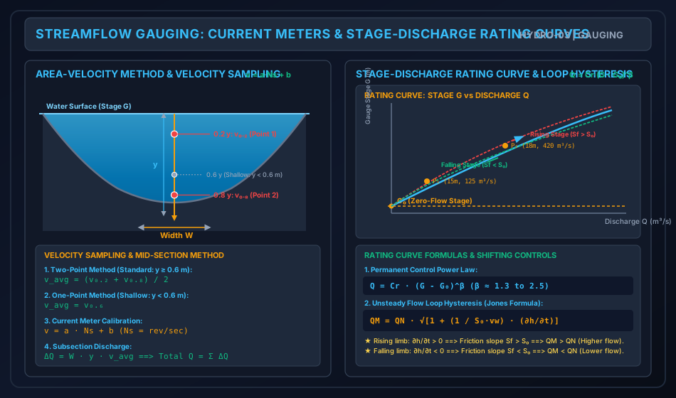
- Vertical-Axis Meter (Price Cup Type): A wheel of six conical cups rotating in a horizontal plane around a vertical spindle. High durability, functions in sediment-laden flows, but tends to over-register in turbulent or oblique flow due to vertical velocity components.
- Horizontal-Axis Meter (Propeller / Ott Type): A streamlined propeller blade rotating in a vertical plane around a horizontal axis parallel to the flow direction. Highly accurate in complex streamlines; unaffected by vertical velocity fluctuations.
Calibration Equation: The rotational speed of the meter rotor (, revolutions per second) is calibrated in a towing tank and obeys the linear relationship:
Where is the hydrodynamic pitch (slope) and is the starting friction velocity.
Standard Depth Sampling Protocols (ISO 748 / IS 1192: 1981): Because vertical velocity profiles in open channels are logarithmic:
- Shallow Streams (): Velocity is measured at a single point located at depth from the free surface (i.e., above the bed).
- Standard / Deep Streams (): Velocity is measured at two points: and depth from the free surface. The mean velocity is the unweighted arithmetic average:
- Turbulent Mountain Rivers: Three-point sampling () or surface floats ().
3.2 Stage-Discharge Rating Curves & Loop Hysteresis
At any stable river cross section controlled by a permanent physical constriction (a rock riffle, channel contraction, or weir), a unique relation exists between stage and discharge :
Where:
- = Observed river stage (m).
- = Gauge reading corresponding to zero discharge (m), determined by the lowest point of the controlling cross section.
- = Effective hydraulic head.
- = Empirical rating constants determined by log-log regression ( typically ranges from to ).
The Unsteady Flow Loop Rating Curve (Jones Formula):
During the passage of a major flood wave, the stage-discharge relationship ceases to be single-valued. For the exact same gauge reading (), the discharge measured during the rising stage is significantly greater than that during the falling stage:
               Unsteady Flood Wave Loop Rating Curve (Hysteresis)

     Stage G
        ▲                      / \
        │                    /     \   Rising Limb (Higher Q: Sf > S₀)
        │                  /         \
        │                /             \
        │              /  Steady Rating  \  Falling Limb (Lower Q: Sf < S₀)
        │            /     Curve (QN)      \
    G₀ ─┴──────────/─────────────────────────► Discharge Q
Physical Hydrodynamic Proof: In steady uniform flow, the friction slope equals the bed slope: . In an unsteady flood wave, by the dynamic Saint-Venant momentum equation:
Neglecting minor convective terms and applying kinematic wave celerity :
According to Manning's or Chezy's equation, discharge scales with :
- Rising Stage (): The flood wave crest approaches, increasing the hydraulic gradient (). Hence, .
- Falling Stage (): Water depth recedes, flattening the hydraulic gradient (). Hence, .
3.3 Anatomy of a Flood Hydrograph
A flood hydrograph resulting from an isolated storm consists of three distinct segments:
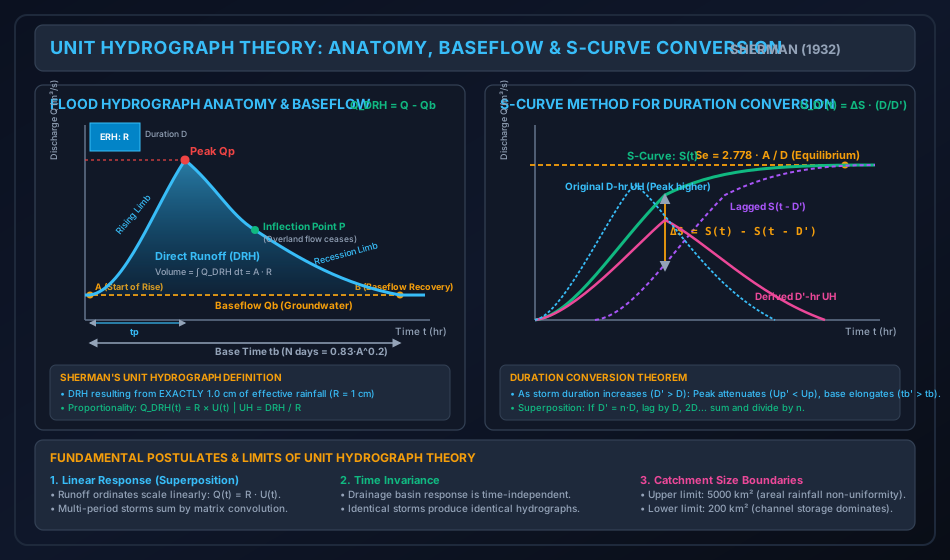
- Rising Limb (Concentration Curve): From the start of direct runoff to the peak. It represents the progressive accumulation of water from increasingly distant tributary zones of the catchment. Its shape is influenced heavily by storm characteristics (intensity, duration, spatial distribution, direction of storm movement).
- Crest Segment: Contains the peak discharge (). It extends from the upper point of inflection on the rising limb to the point of inflection () on the recession limb. The peak discharge occurs when contributing drainage area and rainfall excess intensity reach their combined dynamic maximum.
- Recession Limb (Falling Limb): Extends from the inflection point down to complete baseflow recovery.
- Crucial Physical Property: At the inflection point , all overland sheet flow ceases to enter stream channels. From onward, the hydrograph represents purely the drainage of channel storage and groundwater storage.
- Consequently, the shape of the recession limb is completely independent of storm characteristics; it depends solely on basin geomorphology and channel hydraulics.
- The recession curve follows Barnes' exponential depletion equation: where is the recession constant (typically ).
3.4 Baseflow Separation Techniques
To isolate the Direct Runoff Hydrograph (DRH) from the total flood hydrograph (), three standard techniques are used:
- Method 1: Straight Line Method (Simplest):
- Point is the start of the rising limb.
- Point on the recession limb marks the end of direct runoff, located days after the hydrograph peak.
- Linsley’s empirical equation for duration :
- A straight line connects Point directly to Point . All discharge below line is baseflow; all discharge above is direct runoff.
- Method 2: Two-Line Method:
- The antecedent groundwater recession curve before the storm is projected forward to Point directly under the hydrograph peak.
- Point is then connected by a straight line to Point .
- Method 3: Variable Slope Method:
- The true recession curve after Point is projected backward until it intersects the vertical line drawn through the inflection point at Point .
- A smooth curved transition connects Point to Point .
4. Rigorous Mathematical Formulations & Analytical Derivations
4.1 Proof 1: The Area-Velocity Mid-Section Method
In river cross-section gauging, the channel width is divided into vertical subsections by sounding lines at positions . For any interior vertical with depth and mean velocity :
- The tributary width extends halfway to the adjacent verticals:
- The cross-sectional area of the subsection is:
- The incremental discharge is:
- Total river discharge is the sum across all verticals:
4.2 Proof 2: Direct Runoff Volume & Unit Hydrograph Scaling
The area under the Direct Runoff Hydrograph (DRH) represents the total volume of direct surface water () leaving the catchment:
For discrete discharge data recorded at constant time intervals :
The equivalent depth of direct runoff () distributed uniformly over the catchment area () is:
Derivation of the -hr Unit Hydrograph:
By Sherman’s Principle of Linear Proportionality, the DRH resulting from an effective rainfall depth is simply times the Unit Hydrograph (which represents ):
Unit Conservation Verification Check: The total depth of runoff under the derived Unit Hydrograph MUST identically equal :
4.3 Proof 3: The S-Curve (Summation Curve) Method
The S-Curve (or S-Hydrograph) is defined as the hydrograph of direct surface runoff resulting from a continuous, infinite series of successive -hr unit storms, each producing of effective rainfall at a uniform rate of .
                 Construction of the S-Curve by Summing D-hr UHs

   Discharge Q
        ▲                                                ════════════════════ Se (Equilibrium)
        │                                        . - ~ '
        │                                . - ~ ' ┌───────────────────────────────────────────┐
        │                        . - ~ '         │ Se = 2.778 · A / D                        │
        │                . - ~ '                 └───────────────────────────────────────────┘
        │        . - ~ '
        │  . - ~
        └─────────────────────────────────────────────────────────────────────────────► Time t
           ◄─D─►◄─D─►◄─D─►  (Successive D-hr Unit Hydrographs shifted by D)
Mathematical Formulation:
Let be the ordinates of a -hr Unit Hydrograph. The S-curve ordinate at any time is the sum of the current UH ordinate and all preceding UH ordinates lagged by intervals of :
Derivation of Equilibrium Discharge ():
As time approaches the base length of the Unit Hydrograph, the rate of inflow into the catchment ( every hours) reaches dynamic steady-state equilibrium with the outflow discharge at the outlet:
Where is catchment area in and is the unit storm duration in hours.
Conversion from Duration to Any Arbitrary Duration :
Suppose an S-curve constructed from a -hr UH is lagged by a new desired duration :
- The original S-curve represents continuous rainfall at rate starting at .
- The lagged S-curve represents continuous rainfall at rate starting at .
- The difference between the two S-curves: represents the direct runoff resulting from a rainstorm that lasted for duration at an intensity of .
- Total rainfall depth delivered by this difference storm:
- To reduce this runoff to a Unit Hydrograph of duration (which by definition requires exactly of effective rainfall), we divide the difference by its total depth , which is equivalent to multiplying by the duration ratio :
Key Hydrodynamic Rules of Duration Conversion:
- When (Duration is Increased): The rainfall excess is spread over a longer time at a lower intensity. The peak discharge attenuates (), and the base time elongates ().
- When (Duration is Decreased): The rainfall excess is concentrated into a shorter, sharper burst. The peak discharge increases (), and the base time contracts ().
5. Hand-Coded High-Precision Engineering Visualizations
5.1 Diagram 1: Streamflow Gauging, Current Meters & Rating Curve Loop Hysteresis
The following hand-coded SVG illustrates river discharge measurement using current meter depth sampling protocols ( and ) paired with the stage-discharge rating curve exhibiting unsteady flood wave loop hysteresis (Jones formula).
5.2 Diagram 2: Flood Hydrograph Anatomy, Baseflow & S-Curve Duration Conversion
The following hand-coded SVG details the anatomy of a flood hydrograph, baseflow separation techniques, and the construction of the S-curve to derive Unit Hydrographs of different durations.
6. Comparative Engineering Analysis & Cross-Sectional Synthesis
6.1 Streamflow Velocity Measurement Methods Comparison
| Method | Operating Principle | Applicable Stream Conditions | Accuracy / Standard | Limitations / Failure Modes |
|---|---|---|---|---|
| Current Meter (Cup / Propeller) | Mechanical rotation of rotor; . | Natural rivers, irrigation canals with depths . | Standard benchmark (ISO 748, ). | Weeds/debris foul rotor; dangerous during high flood velocities (). |
| Surface Floats | Measures surface transit time over distance ; . | Unmeasured flash floods, mountain torrents. | Low (). . | Wind drag on floats; surface velocity does not reflect bed shear. |
| Dilution (Tracer) Gauging | Injects known tracer concentration (); measures downstream plateau (). | Turbulent, bouldery mountain streams where cross section cannot be sounded. | High () in steep turbulent reaches. | Requires complete turbulent mixing; tracer adsorption by sediments. |
| Acoustic Doppler (ADCP) | Doppler frequency shift of acoustic pulses reflected off suspended sediment. | Large deep rivers, estuaries, tidal channels. | State of the Art (). Full velocity vector profile. | High equipment cost; fails in pure clear water (no acoustic reflectors). |
6.2 Unit Hydrograph Duration Conversion: Superposition vs S-Curve
| Feature / Comparison | Method of Superposition | S-Curve (Summation Curve) Method |
|---|---|---|
| Permissible Duration Ratio | Strictly Integer Multiples ONLY (, e.g., ). | Completely Universal ( can be any integer, fraction, larger, or smaller, e.g., ). |
| Derivation Mechanism | Lag identical UHs by , sum ordinates, and divide by . | Sum infinite series of -hr UHs to form S-curve, lag by , subtract, and scale by . |
| Computational Effort | Minimal (single tabular addition). | Moderate (requires S-curve tabulation and smoothing). |
| Oscillations / Instability | Perfectly smooth; zero oscillation. | S-curve may oscillate slightly near equilibrium due to discrete tabular rounding; requires graphical smoothing. |
7. Fully Worked Numerical Problems (Pre-Calculated & Verified)
Problem 1: Current Meter River Gauging & Stage-Discharge Rating Curve
Statement: Part A (Velocity Gauging): During streamflow gauging in a river channel, a Price cup current meter was lowered at a vertical sounding station having a total water depth of . The current meter calibration equation is:
Observations recorded:
- At depth below the water surface: The meter registered revolutions in .
- At depth below the water surface: The meter registered revolutions in . The tributary width assigned to this vertical under the mid-section method is .
- Compute the velocities and , and the mean velocity at this vertical.
- Calculate the incremental discharge passing through this subsection.
Part B (Rating Curve Calibration): Hydrologic records at the river gauging station indicate that the stage corresponding to zero discharge is . Two reliable calibration points were established during steady flow conditions:
- Calibration Point 1: River stage , Discharge
- Calibration Point 2: River stage , Discharge
- Formulate the Stage-Discharge Rating Curve equation by evaluating the constants and .
- Predict the flood discharge during an extreme monsoon event when the river gauge rises to .
Step-by-Step Solution:
Part A: Velocity & Incremental Discharge
-
At depth:
-
At depth:
-
Mean velocity at the vertical (standard two-point method for ):
-
Incremental subsection discharge:
Part B: Rating Curve Calibration
Effective heads above zero flow datum :
Setting up the power law ratio:
Taking the natural logarithm:
Evaluating constant from Point 1:
The Authoritative Rating Curve Equation:
Predicting flood discharge at :
Problem 2: Derivation of 4-hr Unit Hydrograph from a Storm Hydrograph
Statement: A catchment of area is subjected to an isolated 4-hour rainstorm. The observed total streamflow discharge at the catchment outlet recorded at regular 6-hour intervals is given below. Stream records show a constant baseflow of .
| Time (hr) | |||||||||||
|---|---|---|---|---|---|---|---|---|---|---|---|
| Total Discharge () |
- Deduce the Direct Runoff Hydrograph (DRH) ordinates by performing straight-line baseflow separation.
- Calculate the total volume of direct surface runoff () in million cubic meters ().
- Determine the equivalent direct runoff depth () in centimeters.
- Derive the ordinates of the 4-hour Unit Hydrograph (4-hr UH).
- State the peak discharge of the 4-hr UH and verify that the derived UH satisfies the unit depth criterion ().
Step-by-Step Solution:
Step 1: Baseflow Separation & DRH Ordinates
Subtract constant baseflow :
- :
- :
- :
- : (Peak of DRH)
- :
- :
- :
- :
- :
- :
- :
Sum of DRH ordinates:
Step 2: Total Runoff Volume ()
Time step .
Step 3: Runoff Depth ()
Catchment area: .
Step 4: 4-hr Unit Hydrograph Ordinates
Divide each DRH ordinate by :
- :
- :
- :
- : (Peak )
- :
- :
- :
- :
- :
- :
- :
Sum of 4-hr UH ordinates:
Step 5: Verification of Unit Runoff Depth
Problem 3: Unit Hydrograph Duration Conversion via S-Curve (4-hr to 8-hr UH)
Statement: The ordinates of a 4-hour Unit Hydrograph for a catchment with an area of are given at 4-hour intervals below:
| Time (hr) | Total | |||||||||
|---|---|---|---|---|---|---|---|---|---|---|
| 4-hr UH () |
Using the S-Curve (Summation curve) method:
- Calculate the theoretical equilibrium discharge of the S-curve () in .
- Tabulate the S-Curve ordinates .
- Tabulate the lagged S-Curve ordinates shifted by the new duration .
- Compute the difference .
- Determine the ordinates of the derived 8-hour Unit Hydrograph ().
- Compare the peak discharge and base time of the 4-hr UH and 8-hr UH.
Step-by-Step Solution:
Step 1: Equilibrium Discharge ()
(Notice that !)
Step 2–5: Tabular S-Curve Construction & 8-hr UH Derivation
Duration ratio multiplier:
| Time (hr) | 4-hr UH () | S-Curve () | S-Curve Lagged by 8 hr | Difference | Derived 8-hr UH () |
|---|---|---|---|---|---|
| 0 | |||||
| 4 | |||||
| 8 | |||||
| 12 | |||||
| 16 | (Peak ) | ||||
| 20 | |||||
| 24 | |||||
| 28 | |||||
| 32 | |||||
| 36 |
Step 6: Engineering Comparison of 4-hr vs 8-hr Unit Hydrographs
- Peak Discharge: Attenuated from (at ) down to (at )—a reduction in peak flood magnitude.
- Time to Peak: Shifted back by 4 hours ().
- Base Time: Elongated from to ().
- Runoff Depth Check:
8. Critical Exam Traps, Failure Modes & Conceptual Pitfalls
   ┌───────────────────────────────────────────────┬───────────────────────────────────────────────┐
   │             EXAM TRAP / MISCONCEPTION         │            RIGOROUS SCIENTIFIC REALITY        │
   ├───────────────────────────────────────────────┼───────────────────────────────────────────────┤
   │ 1. Forgetting to divide DRH by runoff depth R │ TRAP: U(t) = Q_DRH(t) / R. If a storm has    │
   │    when deriving a Unit Hydrograph.           │ R = 3.5 cm, the DRH ordinates MUST be divided│
   │                                               │ by 3.5 to obtain the 1.0-cm Unit Hydrograph.  │
   ├───────────────────────────────────────────────┼───────────────────────────────────────────────┤
   │ 2. Believing a Unit Hydrograph has a unit     │ TRAP: The duration D is NOT 1 hour! A 6-hr UH │
   │    duration of 1.0 hour.                      │ has duration D = 6 hr. The "Unit" refers      │
   │                                               │ EXCLUSIVELY to 1.0 cm of runoff depth!        │
   ├───────────────────────────────────────────────┼───────────────────────────────────────────────┤
   │ 3. Inverting the S-curve scaling factor       │ When converting from D to D', multiply ΔS by  │
   │    as (D' / D) instead of (D / D').           │ (D / D'), NOT (D' / D)! If D' > D, the peak   │
   │                                               │ must be smaller, so D/D' < 1.0.               │
   ├───────────────────────────────────────────────┼───────────────────────────────────────────────┤
   │ 4. Using two-point velocity averaging for a   │ In shallow streams (y < 0.6 m), the current   │
   │    shallow stream with y < 0.6 m.             │ meter CANNOT be submerged to 0.8y. You MUST   │
   │                                               │ use single-point sampling at 0.6y depth.      │
   ├───────────────────────────────────────────────┼───────────────────────────────────────────────┤
   │ 5. Assuming baseflow remains constant during  │ Baseflow typically increases during the flood │
   │    high-stage storms.                         │ peak due to groundwater recharge. Method 1    │
   │                                               │ (straight line) is an engineering convention. │
   ├───────────────────────────────────────────────┼───────────────────────────────────────────────┤
   │ 6. Believing rating curves are fixed forever. │ Rivers experience scour (rating shifts right) │
   │                                               │ and silt deposition (rating shifts left).     │
   │                                               │ Rating curves must be recalibrated regularly. │
   └───────────────────────────────────────────────┴───────────────────────────────────────────────┘
9. Real-World Engineering Case Studies & Forensic Failures
9.1 The Austin Dam Failure (Pennsylvania, USA, 1911)
- Background: The Bayless Pulp and Paper Mill concrete gravity dam on Freeman Run collapsed in September 1911, devastating the downstream town of Austin.
- Hydrologic Failure Mode: Streamflow discharge estimates for spillway sizing were based on intermittent spot staff-gauge readings that completely missed antecedent soil saturation and extreme runoff peaking. When an intense storm occurred, the inflow hydrograph peak severely exceeded the spillway's discharge capacity, overtopping the structure and inducing fatal foundation sliding along weak sandstone strata.
- Remediation: Led to the establishment of permanent state-mandated continuous stream gauging networks and standardized unit hydrograph design guidelines across North America.
9.2 Kerala Floods Hydrograph Inflow Miscalculation (August 2018)
- Background: In August 2018, exceptional monsoon precipitation filled all 35 major reservoirs across Kerala simultaneously, forcing emergency gate openings that exacerbated severe downstream flooding.
- Forensic Finding: A major post-disaster study revealed that several reservoir operations relied on static stage-discharge rating curves that did not account for shifting riverbed controls and severe backwater loop hysteresis. During the rapid flood rise (), actual reservoir inflows were higher than indicated by steady-state gauge tables, delaying controlled gate releases until reservoir surcharge levels were dangerously exceeded.
10. Cross-Disciplinary & Downstream Dependencies
                              ┌──────────────────────────────────────────────┐
                              │  HYDRO-02: Abstractions & φ-Index (ERH)      │
                              └──────────────────────┬───────────────────────┘
                                                     │ Effective Rainfall Depth R & Duration D
                                                     ▼
                              ┌──────────────────────────────────────────────┐
                              │  HYDRO-03: Streamflow, Hydrographs & UH      │
                              │            (S-Curve Conversion & DRH Peak)   │
                              └──────────────────────┬───────────────────────┘
                                                     │ Design Inflow Hydrograph Q(t)
                                                     ▼
                              ┌──────────────────────────────────────────────┐
                              │  HYDRO-04: Reservoir Flood Routing           │
                              │            (Modified Puls) & Gumbel Floods   │
                              └──────────────────────┬───────────────────────┘
                                                     │ Attenuated Spillway Outflow
                                                     ▼
                              ┌──────────────────────────────────────────────┐
                              │  IRRI-03: Ogee Spillway Crest Length &       │
                              │           Stilling Basin Energy Dissipation  │
                              └──────────────────────────────────────────────┘
- Preceding Input:
HYDRO-02computes the Effective Rainfall Hyetograph (ERH) using the -index. - Immediate Successor:
HYDRO-04uses the flood hydrograph derived inHYDRO-03to route flood waves through reservoirs using the Modified Puls storage-indication method, and applies Gumbel’s Extreme Value distribution. - Hydraulic Structures (
IRRI-03/OCF-04): The peak design flood discharge () determined via Unit Hydrograph convolution dictates the spillway crest length, freeboard, and stilling basin dimensions.
11. High-Yield Revision Formula Cheat Sheet
12. Authoritative References & Standards
- Subramanya, K. Engineering Hydrology. 5th ed., McGraw Hill Education (India), 2021. (The authoritative text for Indian civil engineering curriculum and national exams).
- Sherman, L. K. "Streamflow from Rainfall by the Unit-Graph Method." Engineering News-Record, Vol. 108, 1932, pp. 501–505. (The seminal paper founding Unit Hydrograph theory).
- Chow, Ven Te, Maidment, D. R., and Mays, L. W. Applied Hydrology. McGraw-Hill, New York, 1988.
- Bureau of Indian Standards (BIS):
- IS 1192: 1981 (Reaffirmed 2018): Guidelines for Velocity-Area Method for Measurement of Flow of Water in Open Channels.
- IS 1194: 1960 (Reaffirmed 2019): Recommendations for Stage-Discharge Relation for Streamflow Measurement.
- IS 2914: 1964 (Reaffirmed 2019): Recommendations for Estimation of Discharges by Dilution Methods.
- International Organization for Standardization (ISO):
- ISO 748: 2021: Hydrometry - Measurement of Liquid Flow in Open Channels using Current-Meters or Floats.
- Linsley, R. K., Kohler, M. A., and Paulhus, J. L. H. Hydrology for Engineers. McGraw-Hill, New York, 1982.