Numerical Methods, Probability & Mathematical Statistics
In this chapter (1 topics)
On this page
- 1. Executive Summary & Core Definitions
- Core Terminology & Definitions
- 2. Foundational Principles & Governing Axioms
- 2.1 Numerical Root-Finding for Non-Linear Equations
- 2.2 Numerical Integration (Newton-Cotes Closed Quadrature)
- 2.3 Numerical Solution of Initial Value ODEs (y' = f(x, y), y(x0) = y0)
- 2.4 Probability Theory & Governing Axioms
- 2.5 Probability Distributions in Civil Engineering
- 2.6 Descriptive Statistics & Linear Regression
- 3. Step-by-Step Analytical Derivations
- 3.1 Derivation of Quadratic Convergence of Newton-Raphson Method
- 3.2 Derivation of Simpson's 1/3 Rule & Its Cubic Exactness
- 4. Key Formulas & Summary Tables
- 4.1 Master Numerical & Statistical Formulas Reference
- 5. Visual Architectural Diagrams
- 5.1 Numerical Root-Finding, Quadrature & ODE Solvers
- 5.2 Probability Distributions, Characteristic Strength & Statistical Regression
- 6. Standard Practice Guidelines & Boundary Conditions
- 6.1 Limit State Code Compliance (IS 456:2000 & IS 800:2007)
- 6.2 Selection Criteria for Numerical Algorithms
- 7. Critical Failure Modes & Edge Cases
- 7.1 Pathologies of the Newton-Raphson Method
- 7.2 Numerical Quadrature & Runge-Kutta Instabilities
- 8. Worked Numerical Problems
- Problem 1: Newton-Raphson Iteration for Non-Linear Critical Flow Equation
- Problem 2: Comparative Evaluation of Trapezoidal and Simpson's 1/3 Rules
- Problem 3: Hydrological Flood Risk & Limit State Structural Reliability
- 9. Comparative Exam Analysis
- 10. Common Pitfalls & Traps
- 11. Real-World Civil & Structural Applications
- 12. Comprehensive Summary & Quick Revision Guide
- 13. Practice Problems for Self-Assessment
- 14. References & Standard Texts
1. Executive Summary & Core Definitions
Numerical analysis, probability theory, and mathematical statistics provide the essential mathematical machinery for simulating non-linear physical phenomena, evaluating uncertainty, and establishing limit-state reliability across civil engineering infrastructure. Because exact analytical closed-form solutions do not exist for most governing non-linear differential equations and complex physical systems encountered in structural, geotechnical, hydraulic, and environmental engineering, numerical approximations serve as the computational backbone of modern finite element modeling, hydraulic routing, and root-finding solvers. Concurrently, material strength variabilities, seismic ground accelerations, wind gusts, and hydrological extreme events are stochastic in nature; modern limit-state design codes (such as IS 456:2000, IS 800:2007, IS 1893:2016, and IRC 112:2020) are fundamentally founded upon probabilistic characteristic values and semi-probabilistic partial safety factors.
+----------------------------------------------------------------------------------------------------+
|                         ENGINEERING NUMERICAL & STATISTICAL FRAMEWORK                              |
+------------------------------------+-----------------------------------+---------------------------+
|         ROOT-FINDING & ODEs        |        NUMERICAL QUADRATURE       |  PROBABILITY & STATISTICS |
+------------------------------------+-----------------------------------+---------------------------+
| * Bisection Method (Linear, p = 1) | * Trapezoidal Rule [O(h^2)]       | * Axiomatic Probability   |
| * Regula-Falsi (Secant chord)      | * Simpson's 1/3 Rule [O(h^4)]     | * Bayes' Theorem          |
| * Newton-Raphson (Quadratic, p = 2)| * Simpson's 3/8 Rule [O(h^4)]     | * Binomial & Poisson      |
| * Forward Euler [O(h)]             | * Gauss-Legendre Quadrature       | * Normal (Gaussian) Dist. |
| * Runge-Kutta 4th-Order (RK4)      | * Romberg & Adaptive Quadrature   | * Linear Regression & r   |
+------------------------------------+-----------------------------------+---------------------------+
Core Terminology & Definitions
- Order of Convergence (): If an iterative sequence with error satisfies where is the asymptotic error constant, the method has an order of convergence . For , convergence is linear; for , convergence is quadratic (doubling the number of correct decimal places per iteration).
- Newton-Raphson Method: An open root-finding iterative scheme approximating the root of along the tangent line: .
- Newton-Cotes Closed Quadrature: Numerical integration formulas derived by replacing an integrand with an interpolating polynomial passing through equally spaced abscissas.
- Runge-Kutta Methods: A family of single-step explicit numerical solvers for initial value ordinary differential equations () that evaluate slopes at intermediate trial locations to match Taylor series expansions up to an arbitrary order without requiring explicit calculation of higher-order analytical derivatives.
- Sample Space () & Event (): The set of all possible outcomes of a random experiment. An event is a subset of .
- Conditional Probability (): The probability of event occurring given that event has already occurred: , provided .
- Characteristic Strength (): In limit state concrete and steel design, the material strength value below which not more than of test results are expected to fall: , where is the population mean and is the standard deviation.
- Hydrological Return Period (): The average recurrence interval over which an event of given magnitude is equaled or exceeded once. The annual probability of exceedance is .
- Pearson Product-Moment Correlation (): A normalized dimensionless measure of the linear relationship between two continuous variables: .
2. Foundational Principles & Governing Axioms
2.1 Numerical Root-Finding for Non-Linear Equations
Root-finding solves . In civil engineering, this arises in hydraulic normal/critical depth calculations (Manning and Froude equations), foundation settlement equations, and Colebrook-White friction factor equations.
A. Bisection Method (Interval Halving)
- Premise: Based on the Intermediate Value Theorem. If for continuous , at least one root lies within .
- Iterative Scheme: Midpoint . If , root lies in (); otherwise in ().
- Convergence: Strictly guaranteed. Order of convergence (linear).
- Error Bound: After iterations, interval width is . Required iterations for precision :
B. Regula-Falsi (Method of False Position) & Secant Method
- Regula-Falsi: Replaces the curve with a secant chord between bracketed endpoints and : Retains bracket (). Always converges, but order . One endpoint often remains stationary ("stagnation").
- Secant Method: Retains the secant formula but drops the bracketing requirement (). Convergence order is superlinear: . Does not require derivatives, but may diverge.
C. Newton-Raphson Method
- Taylor Series Derivation: Expanding around current estimate :
- Convergence Condition: Sufficient condition for guaranteed local convergence:
- Quadratic Convergence: Let error be . Expanding : Substituting : Thus, order of convergence .
2.2 Numerical Integration (Newton-Cotes Closed Quadrature)
Given , divide into equal subintervals of width , with nodes and ordinates .
+-------------------+---------+-----------------------------------------+---------------------------------+--------------------------+
| METHOD            | STRIPS  | POLYNOMIAL APPROXIMATION                | LOCAL TRUNCATION ERROR          | GLOBAL COMPOSITE ERROR   |
+-------------------+---------+-----------------------------------------+---------------------------------+--------------------------+
| Trapezoidal Rule  | Any n   | Linear segments (Degree 1)              | -(h^3 / 12) f''(xi)             | -((b-a)h^2 / 12) f''(eta)|
| Simpson's 1/3     | Even n  | Quadratic parabolas (Degree 2)          | -(h^5 / 90) f''''(xi)           | -((b-a)h^4 / 180) f''''(n|
| Simpson's 3/8     | Mult. 3 | Cubics through 4 points (Degree 3)      | -(3h^5 / 80) f''''(xi)          | -((b-a)h^4 / 80) f''''(n)|
| Gauss-Legendre    | n pts   | Optimal Legendre orthogonal polynomials | O(h^(2n+1))                     | Exact for deg <= 2n - 1  |
+-------------------+---------+-----------------------------------------+---------------------------------+--------------------------+
A. Trapezoidal Rule
- Connects adjacent ordinates with straight chords:
- Global truncation error: .
- Exact for linear polynomials ().
B. Simpson's 1/3 Rule
- Fits a parabola through sets of three consecutive points over subintervals of width :
- Critical Requirement: The number of subintervals must be even (number of ordinates is odd).
- Global truncation error: .
- Remarkable Property: Although derived using quadratic parabolas (degree 2), the cubic error terms cancel due to symmetry over . Consequently, Simpson's 1/3 rule is exact for polynomials of degree up to 3!
C. Simpson's 3/8 Rule
- Fits a cubic through four points over width . Applicable when is a multiple of 3:
- Global truncation error: .
2.3 Numerical Solution of Initial Value ODEs (, )
A. Forward Euler Method
- Truncates Taylor series after the first derivative:
- Local error: ; Global cumulative error: (First-order accurate). Numerically conditionally stable.
B. Classical Runge-Kutta 4th-Order (RK4) Method
- Computes four weighted slope estimates across the step :
- Local truncation error: ; Global cumulative error: (Fourth-order accurate).
- Self-starting: does not require prior history (unlike multi-step predictor-corrector methods) or analytical evaluation of higher derivatives.
2.4 Probability Theory & Governing Axioms
A. Axioms of Probability (Kolmogorov)
- For any event : .
- For the certain sample space : .
- Countable additivity: If are mutually exclusive ( for ):
B. Key Probability Theorems
- Addition Rule: .
- Multiplication Rule: .
- Independent Events: Events and are statistically independent if and only if .
- Total Probability Theorem: If form a partition of sample space :
- Bayes' Theorem (Inverse Probability):
2.5 Probability Distributions in Civil Engineering
+--------------------+------------+-------------------------------------+-----------------+-----------------------+
| DISTRIBUTION       | TYPE       | PROBABILITY DENSITY / MASS FUNCTION | MEAN (mu)       | VARIANCE (sigma^2)    |
+--------------------+------------+-------------------------------------+-----------------+-----------------------+
| Binomial           | Discrete   | P(X=k) = nCk * p^k * (1-p)^(n-k)    | n * p           | n * p * (1 - p)       |
| Poisson            | Discrete   | P(X=k) = (lambda^k * e^-lambda)/k!  | lambda          | lambda (Var == Mean!) |
| Uniform            | Continuous | f(x) = 1 / (b - a)  for a <= x <= b | (a + b) / 2     | (b - a)^2 / 12        |
| Exponential        | Continuous | f(x) = lambda * e^(-lambda * x)     | 1 / lambda      | 1 / lambda^2          |
| Normal (Gaussian)  | Continuous | f(x) = (1/(sigma*sqrt(2pi)))*e^-... | mu              | sigma^2               |
+--------------------+------------+-------------------------------------+-----------------+-----------------------+
A. Binomial Distribution & Hydrologic Risk
- Describes the number of successes in independent Bernoulli trials with constant probability .
- Hydrological Flood Exceedance: Let be the design return period of an extreme flood.
- Annual exceedance probability: .
- Probability that the flood will not be exceeded in any single year: .
- Probability that the flood will not be exceeded in consecutive years (Reliability / Safety ):
- Probability that the flood will be equaled or exceeded at least once during design life years (Risk ):
B. Poisson Distribution
- Models the count of rare, independent events occurring in a continuous interval of time or space (traffic arrivals at an intersection, annual earthquake occurrences in a seismic zone).
- Limiting form of the Binomial distribution as with .
- Hallmark Property: .
C. Normal (Gaussian) Distribution & Limit State Structural Reliability
- Bell-shaped curve symmetric about mean , with inflection points at .
- Standard Normal Variate: .
- Empirical Rule:
- ()
- ()
- ()
- Characteristic Strength () in IS 456 & IS 800: The 5% defect level corresponds to :
- Characteristic Load (): Load with 95% probability of not being exceeded (upper 5% tail, ):
2.6 Descriptive Statistics & Linear Regression
A. Dispersion & Coefficient of Variation
- Sample Mean:
- Sample Variance:
- Coefficient of Variation (Dimensionless relative variability):
B. Simple Linear Regression (Least Squares Method)
- Model: , where is the fitted line.
- Minimizing sum of squared residuals yields normal equations:
- Regression Coefficients:
- Pearson correlation coefficient:
- Coefficient of Determination: . Represents the proportion of total variance in explained by linear variation in .
3. Step-by-Step Analytical Derivations
3.1 Derivation of Quadratic Convergence of Newton-Raphson Method
Let be the exact root of , so . Let be the approximation at step , with error .
Expanding and using Taylor series about :
Since :
Similarly, expanding the derivative:
Now substitute these into the Newton-Raphson iteration formula:
Subtracting from both sides ():
Using the binomial expansion for small :
Taking limits as :
Conclusion: The error at step is proportional to the square of the error at step . This proves that the Newton-Raphson method possesses quadratic convergence (). If (a multiple root), the expansion breaks down and convergence degrades to linear ().
3.2 Derivation of Simpson's 1/3 Rule & Its Cubic Exactness
Consider three consecutive equally spaced nodes with step size . The corresponding function values are .
Approximate on by a second-degree polynomial:
Integrating analytically from to :
Now express in terms of the ordinates :
- At :
- At :
- At :
Adding and :
Substitute and into the integral formula:
Cubic Exactness Proof: Suppose . The exact integral from to is:
Evaluating via Simpson's 1/3 rule:
The numerical result matches the exact integral identically. Because any general cubic is a linear combination of an odd cubic term and a quadratic polynomial, Simpson's 1/3 rule is identically exact for all polynomials up to degree 3, despite being derived from a quadratic interpolant.
4. Key Formulas & Summary Tables
4.1 Master Numerical & Statistical Formulas Reference
+-------------------------------------------------------------------------------------------------------------------------------+
| TOPIC / METHOD                 | GOVERNING FORMULA                                           | CRITICAL CONSTRAINTS & REMARKS |
+--------------------------------+-------------------------------------------------------------+--------------------------------+
| Newton-Raphson Root Finding    | x_(n+1) = x_n - f(x_n) / f'(x_n)                            | Order p = 2; Fails if f'=0     |
| Secant Method                  | x_(n+1) = x_n - f(x_n)[(x_n - x_(n-1))/(f(x_n)-f(x_(n-1)))] | Order p = 1.618; No derivative |
| Bisection Method               | x_(mid) = (a + b) / 2; n >= log2((b - a) / eps)             | Order p = 1; Always converges  |
| Trapezoidal Rule               | I = (h/2) [y_0 + y_n + 2 sum(y_i)]                          | Error O(h^2); Any n >= 1       |
| Simpson's 1/3 Rule             | I = (h/3) [y_0 + y_n + 4 sum(y_odd) + 2 sum(y_even)]        | Error O(h^4); n MUST BE EVEN   |
| Simpson's 3/8 Rule             | I = (3h/8) [y_0 + y_n + 3(y_1+y_2+y_4+..) + 2(y_3+y_6+..)]  | Error O(h^4); n multiple of 3  |
| 2-Point Gauss-Legendre         | int_{-1}^1 f(t)dt = f(-1/sqrt(3)) + f(1/sqrt(3))            | Exact for polynomials deg <= 3 |
| Forward Euler ODE Solver       | y_(n+1) = y_n + h * f(x_n, y_n)                             | Global Error O(h); 1st Order   |
| Runge-Kutta 4th-Order (RK4)    | y_(n+1) = y_n + (h/6) [k_1 + 2k_2 + 2k_3 + k_4]             | Global Error O(h^4); 4th Order |
| Bayes' Theorem                 | P(B_i|A) = [P(B_i)*P(A|B_i)] / sum[P(B_j)*P(A|B_j)]         | Inverse posterior probability  |
| Binomial Probability           | P(X = k) = nCk * p^k * (1 - p)^(n - k)                      | Mean = np, Var = np(1-p)       |
| Poisson Probability            | P(X = k) = (lambda^k * e^-lambda) / k!                      | Mean = Var = lambda            |
| Hydrologic Flood Risk          | Risk R = 1 - (1 - 1/T)^n; Reliability S = (1 - 1/T)^n       | T = Return period, n = Years   |
| IS 456 Characteristic Strength | f_k = mu - 1.645 * sigma                                    | 5% defective tail (Z = -1.645) |
| IS 456 Characteristic Load     | F_k = mu_L + 1.645 * sigma_L                                | 5% exceedance tail (Z = +1.645) |
| Pearson Correlation (r)        | r = Cov(X, Y) / (sigma_X * sigma_Y)                         | -1 <= r <= +1; R^2 = r^2       |
| Regression Slope (b)           | b = [n sum(xy) - sum(x)sum(y)] / [n sum(x^2) - (sum(x))^2] | b = r * (sigma_Y / sigma_X)    |
| Regression Intercept (a)       | a = y_bar - b * x_bar                                       | Least squares best fit line    |
+-------------------------------------------------------------------------------------------------------------------------------+
5. Visual Architectural Diagrams
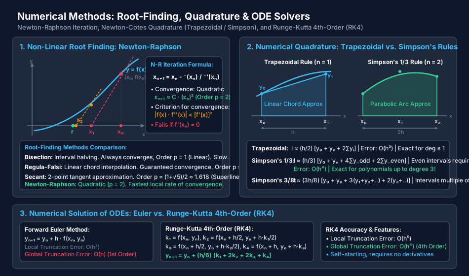
5.1 Numerical Root-Finding, Quadrature & ODE Solvers
The diagram below illustrates the geometric mechanics of the Newton-Raphson tangent sequence, Trapezoidal vs Simpson's 1/3 integration strips, and the multi-slope averaging structure of Runge-Kutta 4th-Order (RK4).
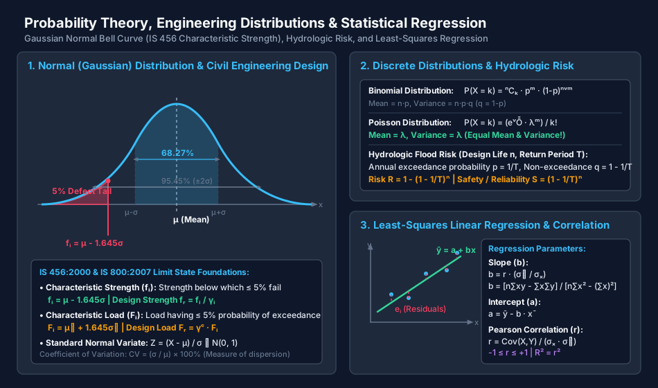
5.2 Probability Distributions, Characteristic Strength & Statistical Regression
The diagram below details the standard Gaussian normal distribution with its coverage, the 5% characteristic strength defect tail () governing IS 456 / IS 800 limit-state design, hydrologic flood risk formulas, and least-squares linear regression.
6. Standard Practice Guidelines & Boundary Conditions
6.1 Limit State Code Compliance (IS 456:2000 & IS 800:2007)
- Concrete Compressive Strength Sampling:
- Under IS 456:2000 Clause 15, characteristic compressive strength is determined from 28-day 150 mm cube tests.
- The design assumes a normal distribution where .
- The partial safety factor for concrete in flexure/compression is , giving design strength: (where the factor accounts for the ratio of structural strength to cube strength).
- Structural Steel Yield Strength Sampling (IS 800:2007):
- Characteristic yield stress reflects the lower 5th percentile: .
- Partial safety factor against yielding: .
- Partial safety factor against ultimate tensile rupture: .
- Acceptance Criteria for Concrete Batches (IS 456 Table 11):
- For M15 or higher: Mean of 4 non-overlapping consecutive test results (or , whichever is greater).
- Individual test result .
6.2 Selection Criteria for Numerical Algorithms
- Root-Finding Selection:
- When derivative is simple to evaluate analytically: Newton-Raphson (fastest, quadratic convergence).
- When function evaluation is computationally expensive or analytical derivative unavailable: Secant Method () or Brent's Method.
- When guaranteed bracketing and safety against divergence is paramount: Bisection Method.
- Quadrature Method Selection:
- For arbitrary discrete field data (survey cross-sections, hydrograph flow ordinates):
- If number of intervals is even: Use Simpson's 1/3 Rule across all strips.
- If number of intervals is odd: Use Simpson's 1/3 Rule for the first strips and apply the Trapezoidal Rule to the final single strip (or combine Simpson's 3/8 for 3 strips and 1/3 for the rest).
- For smooth mathematical functions where evaluation points can be freely chosen: Gauss-Legendre Quadrature gives maximum precision per function evaluation.
- For arbitrary discrete field data (survey cross-sections, hydrograph flow ordinates):
7. Critical Failure Modes & Edge Cases
7.1 Pathologies of the Newton-Raphson Method
- Zero Derivative ():
- If the tangent line becomes parallel to the x-axis, division by zero occurs (). The algorithm terminates with a fatal runtime error.
- Cycle Oscillation (Limit Cycle Trap):
- For functions with symmetric inflection points (e.g., ), an initial estimate gives and , trapping the algorithm in an endless 2-cycle loop that never reaches the true root at .
- Inflection Divergence:
- When initial guess is chosen near an inflection point (), the tangent shoots the next estimate far away from the domain of attraction, resulting in wild divergence.
- Multiple Roots ():
- If root has multiplicity , convergence degrades from quadratic () to linear (). Convergence can be restored to quadratic by using the modified formula:
7.2 Numerical Quadrature & Runge-Kutta Instabilities
- Parity Mismatch in Simpson's 1/3 Rule:
- Attempting to evaluate Simpson's 1/3 rule on an odd number of intervals (even number of ordinates ) is mathematically invalid because parabolas span pairs of intervals (). Applying the formula blindly produces severe errors.
- Step Size () Instability in Forward Euler Method:
- For a stiff linear decay ODE (), Euler's update is . The solution is stable if and only if . If , the numerical solution oscillates with wildly growing exponential amplitude.
8. Worked Numerical Problems
Problem 1: Newton-Raphson Iteration for Non-Linear Critical Flow Equation
A trapezoidal irrigation channel has a discharge equation leading to the non-linear relationship:
where represents the normalized flow depth (in meters).
- Starting with an initial guess , carry out Newton-Raphson iterations until the solution converges to five decimal places.
- Tabulate the iterative sequence showing , , , correction , and verify the quadratic error reduction.
Step-by-Step Analytical Solution
Step 1: Formulate the Derivative
Step 2: Iteration 0 ()
Step 3: Iteration 1 ()
Step 4: Iteration 2 ()
Step 5: Iteration 3 ()
+-----------+------------+---------------+----------------+----------------+
| ITERATION | x_n        | f(x_n)        | f'(x_n)        | Delta x_n      |
+-----------+------------+---------------+----------------+----------------+
| 0         | 2.000000   | -1.000000e+00 | 10.000000      | +0.100000      |
| 1         | 2.100000   | +6.100000e-02 | 11.230000      | -0.005432      |
| 2         | 2.094568   | +1.857232e-04 | 11.161646      | -0.000017      |
| 3         | 2.094551   | +1.739761e-09 | 11.161476      | -1.56e-10      |
+-----------+------------+---------------+----------------+----------------+
Final Answer: The root converged to six decimal places is .
Problem 2: Comparative Evaluation of Trapezoidal and Simpson's 1/3 Rules
A cross-sectional flow profile requires evaluating the definite integral:
- Calculate the exact analytical value.
- Evaluate numerically using the Trapezoidal Rule with step size ( intervals).
- Evaluate numerically using Simpson's 1/3 Rule with ( intervals).
- Compute the absolute and percentage errors for both methods and compare their accuracy.
Step-by-Step Analytical Solution
Step 1: Exact Analytical Evaluation
Step 2: Table of Ordinates (, , interval ) Nodes: . Function: .
+---+-----+---------------+----------------+
| i | x_i | Fraction      | Decimal y_i    |
+---+-----+---------------+----------------+
| 0 | 0.0 | 1 / 1.0       | 1.0000000      |
| 1 | 0.5 | 1 / 1.5 = 2/3 | 0.6666667      |
| 2 | 1.0 | 1 / 2.0 = 1/2 | 0.5000000      |
| 3 | 1.5 | 1 / 2.5 = 2/5 | 0.4000000      |
| 4 | 2.0 | 1 / 3.0 = 1/3 | 0.3333333      |
+---+-----+---------------+----------------+
Step 3: Trapezoidal Rule Calculation
- Absolute Error:
- Percentage Error:
Step 4: Simpson's 1/3 Rule Calculation ( is even )
- Absolute Error:
- Percentage Error:
+--------------------+------------+----------------+------------+
| METHOD             | COMPUTED   | EXACT          | ERROR (%)  |
+--------------------+------------+----------------+------------+
| Trapezoidal (n=4)  | 1.1166667  | 1.0986123      | +1.64%     |
| Simpson's 1/3 (n=4)| 1.1000000  | 1.0986123      | +0.126%    |
+--------------------+------------+----------------+------------+
Comparison: Simpson's 1/3 rule reduces the relative error by a factor of times using the exact same five ordinate points!
Problem 3: Hydrological Flood Risk & Limit State Structural Reliability
A bridge pier on an alluvial river is designed for an economic service life of years.
- If the design flood discharge is assigned a return period of years:
- (a) Compute the probability that this flood will be equaled or exceeded at least once during the 30-year design life (Hydrologic Risk ).
- (b) What return period must be chosen if the client mandates that the total risk of exceedance over 30 years cannot exceed ?
- High-strength deformed steel bars used in the bridge deck have an approximately normal yield strength distribution with population mean and standard deviation .
- (a) Determine the characteristic yield strength according to Indian Standard codes (5% defect level).
- (b) Compute the probability that a randomly sampled bar will have a yield strength strictly less than .
Step-by-Step Analytical Solution
Part 1(a): Flood Risk Calculation for
- Annual exceedance probability:
- Annual non-exceedance probability:
- Hydrologic Reliability (Safety over 30 years): Taking logarithms:
- Hydrologic Risk ():
Part 1(b): Return Period for Over
A design flood with a minimum 300-year return period must be adopted.
Part 2(a): Characteristic Yield Strength ()
- By IS 456 / IS 800 definition, is the 5th percentile value ():
Part 2(b): Probability of Sampling Strength
- Compute the standard normal variate :
- By symmetry of the standard normal distribution: From standard normal CDF tables:
Final Answers:
- Part 1(a): Hydrologic risk
- Part 1(b): Required return period (adopt 300-year flood)
- Part 2(a): Characteristic yield strength
- Part 2(b): Defect probability
9. Comparative Exam Analysis
+------------------+-----------------------------------------------+--------------------------------------------+
| EXAMINATION      | PRIMARY EMPHASIS & RECURRING TOPICS           | CALCULATION FORMAT & PITFALLS              |
+------------------+-----------------------------------------------+--------------------------------------------+
| GATE CE          | * Newton-Raphson quadratic error convergence  | Virtual scientific calculator; Numerical   |
|                  | * Simpson's 1/3 exactness for cubics          | answer type (NAT) requires 2 to 3 decimal  |
|                  | * Runge-Kutta 4th-Order intermediate slopes   | precision; Watch for even interval count!  |
|                  | * Bayes' theorem conditional probability      |                                            |
|                  | * Hydrologic flood risk R = 1 - (1 - 1/T)^n   |                                            |
|                  | * Normal distribution Z-score transformations |                                            |
+------------------+-----------------------------------------------+--------------------------------------------+
| UPSC ESE         | * Analytical proof of quadratic convergence   | Conventional Paper 1: Full algebraic steps |
|                  | * Derivation of Simpson's 1/3 and 3/8 rules   | required; State all intermediate Taylor    |
|                  | * Truncation error comparison and order proof | series expansions and assumptions.         |
|                  | * Characteristic value derivation (fk, Fk)    |                                            |
|                  | * Least-squares regression normal equations   |                                            |
+------------------+-----------------------------------------------+--------------------------------------------+
| SSC JE           | * Definition and order of convergence (p = 2) | Direct factual MCQs; Rapid recall of       |
|                  | * Simpson's 1/3 requires even number of spans | formulas; No negative fractional powers.   |
|                  | * Mean = Variance for Poisson distribution    |                                            |
|                  | * fk = mu - 1.645*sigma definition            |                                            |
+------------------+-----------------------------------------------+--------------------------------------------+
| State AE / JE    | * Error bounds for Trapezoidal vs Simpson     | Formula-based MCQs; Basic 1-step numerical |
|                  | * Euler vs RK4 order comparison (1st vs 4th)  | substitutions without complex calculator.  |
|                  | * Pearson correlation range: -1 <= r <= +1    |                                            |
|                  | * Risk formula: R = 1 - (1 - 1/T)^n           |                                            |
+------------------+-----------------------------------------------+--------------------------------------------+
| RRB JE           | * Basic probability axioms and independent    | Fast arithmetic, straightforward word      |
|                  |   events multiplication rule                  | problems on dice, cards, sampling; Mean,   |
|                  | * Measures of dispersion (CV, variance)       | median, mode empirical relationship.       |
+------------------+-----------------------------------------------+--------------------------------------------+
10. Common Pitfalls & Traps
- Number of Intervals vs. Number of Ordinates:
- In numerical integration, subintervals require ordinates. For Simpson's 1/3 rule, must be even, which means the number of given ordinates must be odd. An exam question giving 10 ordinates has 9 intervals; Simpson's 1/3 rule cannot be applied across all 9 intervals alone!
- Simpson's 1/3 Exactness Degree:
- Because Simpson's 1/3 rule is derived using quadratic parabolas (degree 2), students frequently assume it is only exact for polynomials of degree . Trap: Due to odd-symmetry cancellation over , it is exact for polynomials of degree up to 3!
- Forgetting in Global Error Formulas:
- The local truncation error for Trapezoidal is , but the global composite error across intervals () is . The exponent of drops by 1.
- Equal Mean and Variance Trap:
- If an exam problem states that the mean and variance of a discrete probability distribution are both equal to 4, the distribution is Poisson, not Binomial or Normal.
- Coefficient of Determination ():
- indicates the proportion of explained variance. A correlation produces (). is always non-negative, whereas carries the directional sign of the slope.
11. Real-World Civil & Structural Applications
+----------------------------------------------------------------------------------------------------+
|                         CIVIL ENGINEERING FIELD APPLICATIONS                                       |
+------------------------------------+---------------------------------------------------------------+
| FIELD DOMAIN                       | SPECIFIC NUMERICAL / STATISTICAL IMPLEMENTATION               |
+------------------------------------+---------------------------------------------------------------+
| Structural Engineering (IS 456)    | * Gaussian normal distribution for characteristic concrete    |
|                                    |   strength (fk = mu - 1.645*sigma) and steel yield (fy).      |
|                                    | * Finite element shape functions based on Gauss-Legendre.     |
+------------------------------------+---------------------------------------------------------------+
| Water Resources & Hydrology        | * Flood frequency analysis (Gumbel, Log-Pearson Type III).    |
|                                    | * Hydrologic risk evaluation for dam spillway design lives.   |
|                                    | * Simpson's 1/3 rule for river gauging discharge integration. |
+------------------------------------+---------------------------------------------------------------+
| Geotechnical Engineering           | * Newton-Raphson solution of non-linear consolidation states. |
|                                    | * Statistical reliability index (beta) in slope stability.    |
|                                    | * Trapezoidal rule integration for settlement beneath rafts.  |
+------------------------------------+---------------------------------------------------------------+
| Transportation & Traffic           | * Poisson distribution for vehicle arrivals at toll plazas.   |
|                                    | * Exponential distribution for vehicle headway gaps.          |
|                                    | * Linear regression for travel demand and trip generation.    |
+------------------------------------+---------------------------------------------------------------+
| Environmental Engineering          | * RK4 simulation of dissolved oxygen sag curves (Streeter-P.) |
|                                    | * Bacterial decay modeling via first-order kinetics.          |
+------------------------------------+---------------------------------------------------------------+
12. Comprehensive Summary & Quick Revision Guide
- Newton-Raphson Method: Tangent-based root finder: . Exhibits quadratic convergence (). Fails when .
- Bisection Method: Halves interval where . Order . Slow but guaranteed to converge.
- Trapezoidal Rule: Linear chords: . Error . Exact for degree .
- Simpson's 1/3 Rule: Quadratic parabolic arcs: . Requires even number of subintervals. Error . Exact for polynomials up to degree 3.
- Runge-Kutta 4th-Order (RK4): 4-stage slope averaging: . Local error , global error .
- Hydrological Risk: Probability of exceedance of flood with return period at least once in years: .
- IS Code Characteristic Values: (lower 5% tail); (upper 5% tail).
- Poisson Distribution: Mean = Variance .
- Linear Regression: Best-fit line where and .
13. Practice Problems for Self-Assessment
-
Problem 1: Perform two iterations of the Newton-Raphson method to find the square root of (i.e., solve ) taking .
- Solution: .
- .
- . (Matches to six decimal places).
-
Problem 2: A reservoir cross-section has water depths measured at 1 m intervals (): depths are . Compute the cross-sectional area using Simpson's 1/3 rule.
- Solution: intervals (even ), 7 ordinates ( to ).
- .
- Odd ordinates: .
- Even ordinates: .
- .
-
Problem 3: For a culvert with design service life of 20 years, calculate the risk of failure if designed for a 25-year flood ().
- Solution: . .
-
Problem 4: In a concrete testing program, compressive strength yields and standard deviation . What is the characteristic compressive strength and the coefficient of variation?
- Solution: .
- .
14. References & Standard Texts
- Grewal, B. S., Higher Engineering Mathematics, 44th Edition, Khanna Publishers, New Delhi.
- Chapra, S. C., & Canale, R. P., Numerical Methods for Engineers, 7th Edition, McGraw-Hill Education.
- Jain, M. K., Iyengar, S. R. K., & Jain, R. K., Numerical Methods for Scientific and Engineering Computation, New Age International.
- Kreyszig, E., Advanced Engineering Mathematics, 10th Edition, John Wiley & Sons.
- Walpole, R. E., Myers, R. H., Myers, S. L., & Ye, K., Probability & Statistics for Engineers & Scientists, 9th Edition, Pearson.
- Bureau of Indian Standards (BIS):
- IS 456:2000 - Code of Practice for Plain and Reinforced Concrete.
- IS 800:2007 - General Construction in Steel - Code of Practice.
- IS 1893 (Part 1):2016 - Criteria for Earthquake Resistant Design of Structures.