MATH-03 Chapter 03 · Differential Equations

Ordinary & Partial Differential Equations: Higher-Order Linear ODEs, Cauchy-Euler, Laplace Transforms & Engineering PDEs

1. Executive Summary & Core Definitions

Differential Equations are the mathematical expressions of physical reality across every domain of civil engineering. Whether analyzing the dynamic oscillations of an earthquake-excited bridge deck, the transient consolidation of a soft clay stratum beneath a foundation, the flow net seepage under a concrete dam, or the advective-dispersive transport of contaminants in an urban aquifer, the governing physical laws of mass, momentum, and energy conservation inherently manifest as ordinary or partial differential equations.

Core Terminology & Definitions

  • Ordinary Differential Equation (ODE): An equation containing one or more functions of a single independent variable and its derivatives.
  • Partial Differential Equation (PDE): An equation containing functions of multiple independent variables (e.g., spatial coordinates x,y,zx, y, z and time tt) and their partial derivatives.
  • Order of a Differential Equation: The order of the highest derivative occurring in the equation.
  • Degree of a Differential Equation: The power (exponent) of the highest-order derivative, after the equation has been cleared of radicals and fractions in its derivatives.
  • Linear Differential Equation: A differential equation where the dependent variable and all its derivatives appear strictly in the first degree and are not multiplied together.
  • Exact Differential Equation: A first-order equation M(x,y)dx+N(x,y)dy=0M(x, y) dx + N(x, y) dy = 0 that represents the total differential du=∂u∂xdx+∂u∂ydy=0du = \frac{\partial u}{\partial x} dx + \frac{\partial u}{\partial y} dy = 0 of some scalar function u(x,y)u(x, y).
  • Integrating Factor (IF): A multiplier function μ(x,y)\mu(x, y) that transforms a non-exact differential equation into an exact one, or solves a first-order linear ODE.
  • Complementary Function (CF): The general solution of the associated homogeneous linear differential equation f(D)y=0f(D)y = 0, containing nn arbitrary constants.
  • Particular Integral (PI): Any specific solution of the non-homogeneous equation f(D)y=X(x)f(D)y = X(x) satisfying the driving force without arbitrary constants.
  • Wronskian (WW): The determinant of fundamental solutions and their derivatives W(y1,y2)=y1y2′−y1′y2W(y_1, y_2) = y_1 y_2' - y_1' y_2, utilized in testing linear independence and evaluating particular integrals via variation of parameters.
  • Cauchy-Euler Equation: A linear ODE with variable coefficients where the power of xx in each term matches the order of the derivative: anxndnydxn+⋯+a0y=X(x)a_n x^n \frac{d^n y}{dx^n} + \dots + a_0 y = X(x).
  • Laplace Transform: An integral operational transform mapping a time-domain differential equation f(t)f(t) into a complex frequency-domain algebraic equation F(s)=∫0∞e−stf(t)dtF(s) = \int_0^\infty e^{-st} f(t) dt.

2. Foundational Principles & Governing Axioms

2.1 First-Order Ordinary Differential Equations

  1. Separable Equations: dydx=g(x)h(y)  ⟹  ∫dyh(y)=∫g(x)dx+C\frac{dy}{dx} = g(x) h(y) \implies \int \frac{dy}{h(y)} = \int g(x) dx + C
  2. Exact Differential Equations: M(x,y)dx+N(x,y)dy=0M(x, y) dx + N(x, y) dy = 0
    • Criterion of Exactness: ∂M∂y=∂N∂x\frac{\partial M}{\partial y} = \frac{\partial N}{\partial x}
    • Solution Algorithm: ∫y=constMdx+∫(terms in N free from x)dy=C\int_{y = \text{const}} M dx + \int (\text{terms in } N \text{ free from } x) dy = C
  3. Integrating Factors (IF) for Non-Exact Equations:
    • Case 1 (Function of xx only): If 1N(∂M∂y−∂N∂x)=f(x)  ⟹  IF=e∫f(x)dx\text{If } \frac{1}{N}\left(\frac{\partial M}{\partial y} - \frac{\partial N}{\partial x}\right) = f(x) \implies IF = e^{\int f(x) dx}
    • Case 2 (Function of yy only): If 1M(∂N∂x−∂M∂y)=g(y)  ⟹  IF=e∫g(y)dy\text{If } \frac{1}{M}\left(\frac{\partial N}{\partial x} - \frac{\partial M}{\partial y}\right) = g(y) \implies IF = e^{\int g(y) dy}
  4. First-Order Linear ODE: dydx+P(x)y=Q(x)\frac{dy}{dx} + P(x) y = Q(x) IF=e∫P(x)dxIF = e^{\int P(x) dx} y⋅(IF)=∫[Q(x)⋅(IF)]dx+Cy \cdot (IF) = \int [Q(x) \cdot (IF)] dx + C
  5. Bernoulli's Equation (Non-Linear): dydx+P(x)y=Q(x)yn(n≠0,1)\frac{dy}{dx} + P(x) y = Q(x) y^n \quad (n \neq 0, 1) Dividing across by yny^n: y−ndydx+P(x)y1−n=Q(x)y^{-n} \frac{dy}{dx} + P(x) y^{1-n} = Q(x). Substituting v=y1−n  ⟹  dvdx=(1−n)y−ndydxv = y^{1-n} \implies \frac{dv}{dx} = (1 - n) y^{-n} \frac{dy}{dx}, reducing the equation to linear: dvdx+(1−n)P(x)v=(1−n)Q(x)\frac{dv}{dx} + (1 - n) P(x) v = (1 - n) Q(x)

2.2 Higher-Order Linear ODEs with Constant Coefficients

General form:

dnydxn+an−1dn−1ydxn−1+⋯+a1dydx+a0y=X(x)\frac{d^n y}{dx^n} + a_{n-1} \frac{d^{n-1}y}{dx^{n-1}} + \dots + a_1 \frac{dy}{dx} + a_0 y = X(x)

Written in operator notation (D=ddxD = \frac{d}{dx}):

f(D)y=X(x)f(D) y = X(x)

Complete Solution:

y(x)=yc(x)+yp(x)=CF+PIy(x) = y_c(x) + y_p(x) = \text{CF} + \text{PI}

A. Complementary Function (CF) via Auxiliary Equation f(m)=0f(m) = 0:

  1. Real & Distinct Roots (m1≠m2m_1 \neq m_2): yc=c1em1x+c2em2xy_c = c_1 e^{m_1 x} + c_2 e^{m_2 x}
  2. Real & Repeated Roots (m1=m2=mm_1 = m_2 = m): yc=(c1+c2x)emxy_c = (c_1 + c_2 x) e^{m x} (For kk repeated roots: (c1+c2x+⋯+ckxk−1)emx(c_1 + c_2 x + \dots + c_k x^{k-1})e^{mx})
  3. Complex Conjugate Roots (m=α±iβm = \alpha \pm i \beta): yc=eαx(c1cos⁡βx+c2sin⁡βx)y_c = e^{\alpha x} (c_1 \cos\beta x + c_2 \sin\beta x)
  4. Repeated Complex Conjugate Roots (m=α±iβm = \alpha \pm i \beta twice): yc=eαx[(c1+c2x)cos⁡βx+(c3+c4x)sin⁡βx]y_c = e^{\alpha x} \left[(c_1 + c_2 x)\cos\beta x + (c_3 + c_4 x)\sin\beta x\right]

B. Particular Integral (PI) Operator Rules (yp=1f(D)Xy_p = \frac{1}{f(D)} X):

  1. Exponential X=eaxX = e^{ax}: 1f(D)eax=1f(a)eaxprovided f(a)≠0\frac{1}{f(D)} e^{ax} = \frac{1}{f(a)} e^{ax} \quad \text{provided } f(a) \neq 0 If f(a)=0f(a) = 0 (Case of Failure / Resonance): 1f(D)eax=x⋅1f′(D)eax=xf′(a)eax\frac{1}{f(D)} e^{ax} = x \cdot \frac{1}{f'(D)} e^{ax} = \frac{x}{f'(a)} e^{ax}
  2. Trigonometric X=sin⁡(ax)X = \sin(ax) or cos⁡(ax)\cos(ax): Replace D2D^2 with −a2-a^2 in f(D2)f(D^2): 1ϕ(D2)sin⁡(ax)=1ϕ(−a2)sin⁡(ax)provided ϕ(−a2)≠0\frac{1}{\phi(D^2)} \sin(ax) = \frac{1}{\phi(-a^2)} \sin(ax) \quad \text{provided } \phi(-a^2) \neq 0 If ϕ(−a2)=0\phi(-a^2) = 0: 1D2+a2sin⁡(ax)=−x2acos⁡(ax),1D2+a2cos⁡(ax)=x2asin⁡(ax)\frac{1}{D^2 + a^2} \sin(ax) = -\frac{x}{2a}\cos(ax), \quad \frac{1}{D^2 + a^2} \cos(ax) = \frac{x}{2a}\sin(ax)
  3. Polynomial X=xmX = x^m: Expand [f(D)]−1[f(D)]^{-1} as an ascending binomial power series in DD up to order DmD^m.
  4. Product X=eaxV(x)X = e^{ax} V(x) (Exponential Shift): 1f(D)[eaxV(x)]=eax1f(D+a)V(x)\frac{1}{f(D)} [e^{ax} V(x)] = e^{ax} \frac{1}{f(D + a)} V(x)

3. Step-by-Step Analytical Derivations

3.1 Method of Variation of Parameters

Consider the general 2nd-order non-homogeneous linear ODE:

y′′+P(x)y′+Q(x)y=X(x)y'' + P(x) y' + Q(x) y = X(x)

Let y1(x)y_1(x) and y2(x)y_2(x) be two linearly independent solutions of the homogeneous equation y′′+Py′+Qy=0y'' + P y' + Q y = 0. The complementary function is yc=c1y1+c2y2y_c = c_1 y_1 + c_2 y_2. In variation of parameters, we replace constants c1,c2c_1, c_2 with unknown variable functions u1(x),u2(x)u_1(x), u_2(x):

yp(x)=u1(x)y1(x)+u2(x)y2(x)y_p(x) = u_1(x) y_1(x) + u_2(x) y_2(x)

Differentiating:

yp′=(u1′y1+u2′y2)+(u1y1′+u2y2′)y_p' = (u_1' y_1 + u_2' y_2) + (u_1 y_1' + u_2 y_2')

To simplify, we enforce the first constraint:

u1′y1+u2′y2=0— (Constraint 1)u_1' y_1 + u_2' y_2 = 0 \quad \text{--- (Constraint 1)}

Then yp′=u1y1′+u2y2′y_p' = u_1 y_1' + u_2 y_2'. Differentiating again:

yp′′=u1′y1′+u2′y2′+u1y1′′+u2y2′′y_p'' = u_1' y_1' + u_2' y_2' + u_1 y_1'' + u_2 y_2''

Substituting yp,yp′,yp′′y_p, y_p', y_p'' into the ODE:

(u1′y1′+u2′y2′+u1y1′′+u2y2′′)+P(u1y1′+u2y2′)+Q(u1y1+u2y2)=X(x)(u_1' y_1' + u_2' y_2' + u_1 y_1'' + u_2 y_2'') + P(u_1 y_1' + u_2 y_2') + Q(u_1 y_1 + u_2 y_2) = X(x) u1(y1′′+Py1′+Qy1)+u2(y2′′+Py2′+Qy2)+(u1′y1′+u2′y2′)=X(x)u_1(y_1'' + P y_1' + Q y_1) + u_2(y_2'' + P y_2' + Q y_2) + (u_1' y_1' + u_2' y_2') = X(x)

Since y1,y2y_1, y_2 solve the homogeneous equation, the first two terms vanish:

u1′y1′+u2′y2′=X(x)— (Constraint 2)u_1' y_1' + u_2' y_2' = X(x) \quad \text{--- (Constraint 2)}

We now have a system of two algebraic equations in u1′,u2′u_1', u_2':

[y1y2y1′y2′]{u1′u2′}={0X(x)}\begin{bmatrix} y_1 & y_2 \\ y_1' & y_2' \end{bmatrix} \begin{Bmatrix} u_1' \\ u_2' \end{Bmatrix} = \begin{Bmatrix} 0 \\ X(x) \end{Bmatrix}

The determinant of this system is the Wronskian:

W=det⁡[y1y2y1′y2′]=y1y2′−y1′y2W = \det\begin{bmatrix} y_1 & y_2 \\ y_1' & y_2' \end{bmatrix} = y_1 y_2' - y_1' y_2

Applying Cramer's rule:

u1′=∣0y2Xy2′∣W=−y2XW  ⟹  u1(x)=−∫y2XWdxu_1' = \frac{\begin{vmatrix} 0 & y_2 \\ X & y_2' \end{vmatrix}}{W} = -\frac{y_2 X}{W} \implies u_1(x) = -\int \frac{y_2 X}{W} dx u2′=∣y10y1′X∣W=y1XW  ⟹  u2(x)=∫y1XWdxu_2' = \frac{\begin{vmatrix} y_1 & 0 \\ y_1' & X \end{vmatrix}}{W} = \frac{y_1 X}{W} \implies u_2(x) = \int \frac{y_1 X}{W} dx

Final Particular Integral Formula:

yp(x)=−y1(x)∫y2(x)X(x)W(x)dx+y2(x)∫y1(x)X(x)W(x)dxy_p(x) = -y_1(x) \int \frac{y_2(x) X(x)}{W(x)} dx + y_2(x) \int \frac{y_1(x) X(x)}{W(x)} dx

3.2 Classification of Second-Order Partial Differential Equations

The general semi-linear second-order PDE in two independent variables (x,y)(x, y) is:

A∂2u∂x2+B∂2u∂x∂y+C∂2u∂y2+D∂u∂x+E∂u∂y+Fu=G(x,y)A \frac{\partial^2 u}{\partial x^2} + B \frac{\partial^2 u}{\partial x \partial y} + C \frac{\partial^2 u}{\partial y^2} + D \frac{\partial u}{\partial x} + E \frac{\partial u}{\partial y} + F u = G(x, y)

To classify its mathematical character, consider characteristic coordinates ξ(x,y)\xi(x, y) and η(x,y)\eta(x, y). Transforming the second derivatives:

Auxx+Buxy+Cuyy=[Aξx2+Bξxξy+Cξy2]uξξ+…A u_{xx} + B u_{xy} + C u_{yy} = [A \xi_x^2 + B \xi_x \xi_y + C \xi_y^2] u_{\xi\xi} + \dots

Setting the leading characteristic coefficient to zero:

A(dydx)2−B(dydx)+C=0A \left(\frac{dy}{dx}\right)^2 - B \left(\frac{dy}{dx}\right) + C = 0

The roots of the characteristic equation are:

dydx=B±B2−4AC2A\frac{dy}{dx} = \frac{B \pm \sqrt{B^2 - 4AC}}{2A}

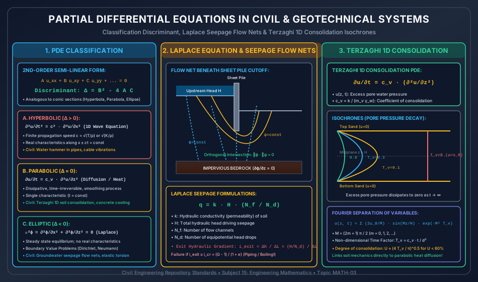
The nature of these characteristic curves depends strictly on the Discriminant Δ=B2−4AC\Delta = B^2 - 4AC:

                              Discriminant Δ = B² - 4AC
                                         │
                 ┌───────────────────────┼───────────────────────┐
                 │                       │                       │
               Δ > 0                   Δ = 0                   Δ < 0
                 │                       │                       │
            HYPERBOLIC               PARABOLIC               ELLIPTIC
        Two Real Curves         One Real Curve          No Real Curves
     (1D Wave Equation)       (Heat/Consolidation)     (Laplace/Poisson)
  1. Hyperbolic (Δ=B2−4AC>0\Delta = B^2 - 4AC > 0):
    • Two families of distinct real characteristic curves along which disturbances propagate at finite speed.
    • Example: 1D Wave equation ∂2u∂t2−c2∂2u∂x2=0  ⟹  A=1,B=0,C=−c2  ⟹  Δ=0−4(1)(−c2)=4c2>0\frac{\partial^2 u}{\partial t^2} - c^2 \frac{\partial^2 u}{\partial x^2} = 0 \implies A = 1, B = 0, C = -c^2 \implies \Delta = 0 - 4(1)(-c^2) = 4c^2 > 0.
  2. Parabolic (Δ=B2−4AC=0\Delta = B^2 - 4AC = 0):
    • One family of real characteristic curves; represents time-dependent diffusive processes.
    • Example: Terzaghi 1D consolidation equation ∂u∂t−cv∂2u∂z2=0  ⟹  A=−cv,B=0,C=0  ⟹  Δ=0\frac{\partial u}{\partial t} - c_v \frac{\partial^2 u}{\partial z^2} = 0 \implies A = -c_v, B = 0, C = 0 \implies \Delta = 0.
  3. Elliptic (Δ=B2−4AC<0\Delta = B^2 - 4AC < 0):
    • No real characteristics; disturbances propagate instantaneously in all directions; represents static equilibrium.
    • Example: 2D Laplace equation ∂2ϕ∂x2+∂2ϕ∂z2=0  ⟹  A=1,B=0,C=1  ⟹  Δ=0−4(1)(1)=−4<0\frac{\partial^2 \phi}{\partial x^2} + \frac{\partial^2 \phi}{\partial z^2} = 0 \implies A = 1, B = 0, C = 1 \implies \Delta = 0 - 4(1)(1) = -4 < 0.

4. Key Formulas & Summary Tables

4.1 Master Differential Equations Formula Table

Equation Type Standard Form Method of Solution / Governing Result
Exact 1st-Order Mdx+Ndy=0M dx + N dy = 0 (∂M∂y=∂N∂x\frac{\partial M}{\partial y} = \frac{\partial N}{\partial x}) ∫y=cMdx+∫(terms in N free from x)dy=C\int_{y=c} M dx + \int (\text{terms in } N \text{ free from } x) dy = C
Linear 1st-Order y′+P(x)y=Q(x)y' + P(x) y = Q(x) IF=e∫Pdx  ⟹  y⋅IF=∫(Q⋅IF)dx+CIF = e^{\int P dx} \implies y \cdot IF = \int (Q \cdot IF) dx + C
Bernoulli ODE y′+Py=Qyny' + P y = Q y^n Substitute v=y1−n  ⟹  v′+(1−n)Pv=(1−n)Qv = y^{1-n} \implies v' + (1-n) P v = (1-n) Q
Cauchy-Euler x2y′′+a1xy′+a0y=Xx^2 y'' + a_1 x y' + a_0 y = X x=ez  ⟹  xD=Dz,x2D2=Dz(Dz−1)x = e^z \implies x D = D_z, x^2 D^2 = D_z(D_z - 1)
Wronskian W(y1,y2)=y1y2′−y1′y2W(y_1, y_2) = y_1 y_2' - y_1' y_2 W≠0W \neq 0 for linear independence; variation of parameters
Laplace 1st Deriv L{f′(t)}=sF(s)−f(0)\mathcal{L}\{f'(t)\} = s F(s) - f(0) Eliminates derivatives; algebraic transformation of IVPs
Laplace 2nd Deriv L{f′′(t)}=s2F(s)−sf(0)−f′(0)\mathcal{L}\{f''(t)\} = s^2 F(s) - s f(0) - f'(0) Solves 2nd-order dynamic vibration IVPs directly
PDE Discriminant Δ=B2−4AC\Delta = B^2 - 4AC Δ>0\Delta > 0: Hyperbolic | Δ=0\Delta = 0: Parabolic | Δ<0\Delta < 0: Elliptic
Seepage Discharge q=kHNfNdq = k H \frac{N_f}{N_d} Flownet solution of 2D Laplace PDE ∇2h=0\nabla^2 h = 0
Terzaghi PDE ∂u∂t=cv∂2u∂z2\frac{\partial u}{\partial t} = c_v \frac{\partial^2 u}{\partial z^2} Time factor Tv=cvtd2T_v = \frac{c_v t}{d^2}; excess pore pressure dissipation

5. Visual Architectural Diagrams

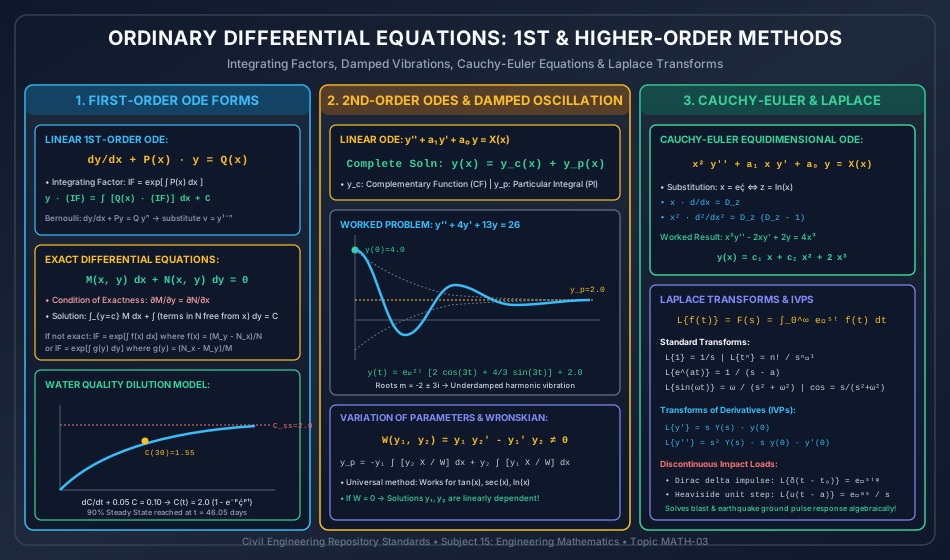
5.1 Ordinary Differential Equations Methods & Solutions

Ordinary Differential Equations Methods and Solutions

5.2 PDE Classification & Civil Engineering Boundary Value Problems

PDE Classification and Boundary Value Problems

6. Standard Practice Guidelines & Boundary Conditions

6.1 Initial vs Boundary Value Problems

  1. Initial Value Problems (IVPs):
    • All auxiliary conditions are specified at a single point (typically t=0t = 0: displacement y(0)y(0) and velocity y′(0)y'(0)).
    • Solved with Laplace transforms or classical complementary/particular integrals.
  2. Boundary Value Problems (BVPs):
    • Conditions are specified at two or more spatial boundaries (e.g., beam deflection y(0)=0y(0) = 0 at left support, y(L)=0y(L) = 0 at right support).
    • Generates eigenvalue problems (e.g., Euler buckling loads Pcr=π2EIL2P_{cr} = \frac{\pi^2 EI}{L^2}).

6.2 Types of Boundary Conditions in PDEs

  1. Dirichlet Boundary Condition:
    • The value of the unknown function is explicitly prescribed along the boundary: u∣Γ=f(x,y)u|_{\Gamma} = f(x, y)
    • Civil Example: Prescribed hydraulic head along upstream river bed (h=Hh = H) in dam seepage.
  2. Neumann Boundary Condition:
    • The normal gradient (derivative) is prescribed along the boundary: ∂u∂n∣Γ=g(x,y)\left.\frac{\partial u}{\partial n}\right|_{\Gamma} = g(x, y)
    • Civil Example: Impermeable bedrock base where ∂h∂z=0\frac{\partial h}{\partial z} = 0 (zero normal flow).
  3. Robin / Mixed Boundary Condition:
    • Linear combination of value and normal derivative: (αu+β∂u∂n)∣Γ=h(x,y)\left.\left(\alpha u + \beta \frac{\partial u}{\partial n}\right)\right|_{\Gamma} = h(x, y)
    • Civil Example: Heat convection from curing concrete into ambient air.

7. Critical Failure Modes & Edge Cases

  1. Resonance Phenomenon in Forced Oscillations:
    • If driving frequency matches natural frequency (Ω=ωn\Omega = \omega_n), the denominator in the particular integral 1D2+ωn2sin⁡(ωnt)\frac{1}{D^2 + \omega_n^2} \sin(\omega_n t) vanishes (f(a)=0f(a) = 0).
    • The particular integral becomes yp(t)=−t2ωncos⁡(ωnt)y_p(t) = -\frac{t}{2\omega_n} \cos(\omega_n t), growing linearly without bound   ⟹  \implies catastrophic structural collapse (e.g., Broughton Suspension Bridge, Millennium Bridge lateral resonance).
  2. Singular Points in Cauchy-Euler Equations:
    • The point x=0x = 0 is a regular singular point. Cauchy-Euler solutions y=c1xm1+c2xm2y = c_1 x^{m_1} + c_2 x^{m_2} can blow up at x=0x = 0 if roots are negative. Boundary conditions must be applied strictly for x>0x > 0.
  3. Piping Failure from Flownet Exit Gradients:
    • In 2D Laplace seepage, if the exit hydraulic gradient iexit=ΔhΔL≥icr=G−11+ei_{\text{exit}} = \frac{\Delta h}{\Delta L} \ge i_{cr} = \frac{G - 1}{1 + e}, effective stress drops to zero. Soil boiling and backward erosion piping undermine the dam foundation.

8. Worked Numerical Problems

Problem 1: First-Order Linear ODE Governing Environmental Reservoir Dilution

Statement:
A municipal water storage reservoir of constant volume V=1000.00 m3V = 1000.00\text{ m}^3 receives an industrial discharge inflow at a constant volumetric rate Q=20.00 m3/dayQ = 20.00\text{ m}^3/\text{day} with a constant contaminant concentration Cin=5.00 mg/LC_{\text{in}} = 5.00\text{ mg/L}.
The well-mixed reservoir discharges treated water at the same rate Q=20.00 m3/dayQ = 20.00\text{ m}^3/\text{day}. Inside the reservoir, the pollutant undergoes first-order biochemical decay with a reaction rate constant k=0.03 day−1k = 0.03\text{ day}^{-1}.
Assuming the reservoir is initially clean (C(0)=0.00 mg/LC(0) = 0.00\text{ mg/L}):

  1. Formulate the governing differential equation and find the integrating factor.
  2. Determine the analytical expression for pollutant concentration C(t)C(t) as a function of time.
  3. Calculate the steady-state concentration (CssC_{\text{ss}}) as t→∞t \to \infty.
  4. Calculate the concentration at t=30.00 dayst = 30.00\text{ days}.
  5. Calculate the time required for the concentration to reach 90.00%90.00\% of its steady-state value.

Step-by-Step Analytical Solution

Part 1: Governing ODE Formulation & Integrating Factor Mass conservation rate equation:

Rate of Mass Accumulation=Mass Inflow Rate−Mass Outflow Rate−Decay Rate\text{Rate of Mass Accumulation} = \text{Mass Inflow Rate} - \text{Mass Outflow Rate} - \text{Decay Rate} VdCdt=QCin−QC(t)−kVC(t)V \frac{dC}{dt} = Q C_{\text{in}} - Q C(t) - k V C(t)

Dividing through by volume VV:

dCdt+(QV+k)C(t)=QCinV\frac{dC}{dt} + \left(\frac{Q}{V} + k\right) C(t) = \frac{Q C_{\text{in}}}{V}

Substituting parameter values:

  • QV=20.001000.00=0.02 day−1\frac{Q}{V} = \frac{20.00}{1000.00} = 0.02\text{ day}^{-1}
  • Total rate coefficient: P=QV+k=0.02+0.03=0.05 day−1P = \frac{Q}{V} + k = 0.02 + 0.03 = \mathbf{0.05\text{ day}^{-1}}
  • Source term: Qterm=QCinV=0.02×5.00=0.10 mg/(L⋅day)Q_{\text{term}} = \frac{Q C_{\text{in}}}{V} = 0.02 \times 5.00 = \mathbf{0.10\text{ mg}/(\text{L}\cdot\text{day})}

Standard linear 1st-order form:

dCdt+0.05C=0.10\frac{dC}{dt} + 0.05 C = 0.10

Integrating Factor (IFIF):

IF=e∫0.05dt=e0.05tIF = e^{\int 0.05 dt} = \mathbf{e^{0.05 t}}

Part 2: Analytical Solution for C(t)C(t) Multiplying by IFIF:

C(t)⋅e0.05t=∫0.10e0.05tdt+C0=0.100.05e0.05t+C0=2.00e0.05t+C0C(t) \cdot e^{0.05 t} = \int 0.10 e^{0.05 t} dt + C_0 = \frac{0.10}{0.05} e^{0.05 t} + C_0 = 2.00 e^{0.05 t} + C_0

Dividing by e0.05te^{0.05 t}:

C(t)=2.00+C0e−0.05tC(t) = 2.00 + C_0 e^{-0.05 t}

Applying initial condition C(0)=0.00C(0) = 0.00:

0.00=2.00+C0  ⟹  C0=−2.000.00 = 2.00 + C_0 \implies C_0 = -2.00 C(t)=2.00(1−e−0.05t) mg/L\mathbf{C(t) = 2.00 \left(1 - e^{-0.05 t}\right)\text{ mg/L}}

Part 3: Steady-State Concentration (CssC_{\text{ss}}) As t→∞t \to \infty, e−0.05t→0e^{-0.05 t} \to 0:

Css=2.00 mg/LC_{\text{ss}} = \mathbf{2.00\text{ mg/L}}

Part 4: Concentration at t=30.00 dayst = 30.00\text{ days}

C(30)=2.00(1−e−0.05×30)=2.00(1−e−1.50)C(30) = 2.00 \left(1 - e^{-0.05 \times 30}\right) = 2.00 \left(1 - e^{-1.50}\right) e−1.50=0.223130e^{-1.50} = 0.223130 C(30)=2.00×(1−0.223130)=2.00×0.776870=1.5537 mg/LC(30) = 2.00 \times (1 - 0.223130) = 2.00 \times 0.776870 = \mathbf{1.5537\text{ mg/L}}

Part 5: Time to Reach 90%90\% of Steady State

C(t)=0.90×Css=0.90×2.00=1.80 mg/LC(t) = 0.90 \times C_{\text{ss}} = 0.90 \times 2.00 = 1.80\text{ mg/L} 2.00(1−e−0.05t)=1.80  ⟹  1−e−0.05t=0.90  ⟹  e−0.05t=0.102.00 \left(1 - e^{-0.05 t}\right) = 1.80 \implies 1 - e^{-0.05 t} = 0.90 \implies e^{-0.05 t} = 0.10 −0.05t=ln⁡(0.10)=−2.302585-0.05 t = \ln(0.10) = -2.302585 t=2.3025850.05=46.05 dayst = \frac{2.302585}{0.05} = \mathbf{46.05\text{ days}}

Problem 2: Second-Order Linear ODE with Constant Coefficients (Damped SDOF Dynamic Response)

Statement:
The lateral dynamic displacement y(t)y(t) of an elevated structural frame subjected to a step blast wind overpressure is governed by the second-order differential equation:

d2ydt2+4dydt+13y=26\frac{d^2 y}{dt^2} + 4\frac{dy}{dt} + 13 y = 26

Subject to initial conditions: at t=0t = 0, displacement y(0)=4.00 mmy(0) = 4.00\text{ mm}, and initial velocity y′(0)=0.00 mm/sy'(0) = 0.00\text{ mm/s}.

  1. Find the roots of the auxiliary equation and write the Complementary Function (yc(t)y_c(t)).
  2. Calculate the Particular Integral (yp(t)y_p(t)).
  3. Determine the complete analytical solution y(t)y(t) satisfying both initial conditions.
  4. Calculate the displacement at time t=1.00 st = 1.00\text{ s}.

Step-by-Step Analytical Solution

Part 1: Auxiliary Equation & Complementary Function Auxiliary equation:

m2+4m+13=0m^2 + 4m + 13 = 0

Using the quadratic formula:

m=−4±42−4(1)(13)2(1)=−4±16−522=−4±−362=−2±3im = \frac{-4 \pm \sqrt{4^2 - 4(1)(13)}}{2(1)} = \frac{-4 \pm \sqrt{16 - 52}}{2} = \frac{-4 \pm \sqrt{-36}}{2} = -2 \pm 3i

The roots are complex conjugate: α=−2.00\alpha = -2.00, β=3.00 rad/s\beta = 3.00\text{ rad/s}. The complementary function represents exponentially decaying harmonic oscillation:

yc(t)=e−2t(c1cos⁡3t+c2sin⁡3t)y_c(t) = e^{-2t} \left(c_1 \cos 3t + c_2 \sin 3t\right)

Part 2: Particular Integral (ypy_p) Since X(t)=26X(t) = 26 (constant):

yp=1D2+4D+13(26)=2613=2.00 mmy_p = \frac{1}{D^2 + 4D + 13}(26) = \frac{26}{13} = \mathbf{2.00\text{ mm}}

Part 3: Complete Solution & Evaluation of Constants

y(t)=yc(t)+yp=e−2t(c1cos⁡3t+c2sin⁡3t)+2.00y(t) = y_c(t) + y_p = e^{-2t} \left(c_1 \cos 3t + c_2 \sin 3t\right) + 2.00

Applying y(0)=4.00y(0) = 4.00:

y(0)=e0(c1cos⁡0+0)+2.00=c1+2.00=4.00  ⟹  c1=2.00y(0) = e^0 (c_1 \cos 0 + 0) + 2.00 = c_1 + 2.00 = 4.00 \implies \mathbf{c_1 = 2.00}

Differentiating y(t)y(t):

y′(t)=−2e−2t(c1cos⁡3t+c2sin⁡3t)+e−2t(−3c1sin⁡3t+3c2cos⁡3t)y'(t) = -2 e^{-2t} \left(c_1 \cos 3t + c_2 \sin 3t\right) + e^{-2t} \left(-3 c_1 \sin 3t + 3 c_2 \cos 3t\right)

Applying y′(0)=0.00y'(0) = 0.00:

y′(0)=−2(c1)+3c2=−2(2.00)+3c2=−4.00+3c2=0  ⟹  3c2=4.00  ⟹  c2=43≈1.3333y'(0) = -2(c_1) + 3 c_2 = -2(2.00) + 3 c_2 = -4.00 + 3 c_2 = 0 \implies 3 c_2 = 4.00 \implies \mathbf{c_2 = \frac{4}{3} \approx 1.3333}

Complete exact analytical solution:

y(t)=e−2t(2.00cos⁡3t+43sin⁡3t)+2.00 mm\mathbf{y(t) = e^{-2t} \left(2.00 \cos 3t + \frac{4}{3} \sin 3t\right) + 2.00\text{ mm}}

Part 4: Displacement at t=1.00 st = 1.00\text{ s}

cos⁡(3.00 rad)=−0.989992,sin⁡(3.00 rad)=0.141120\cos(3.00\text{ rad}) = -0.989992, \quad \sin(3.00\text{ rad}) = 0.141120 2.00(−0.989992)+1.333333(0.141120)=−1.979984+0.188160=−1.7918242.00(-0.989992) + 1.333333(0.141120) = -1.979984 + 0.188160 = -1.791824 e−2(1.00)=e−2=0.135335e^{-2(1.00)} = e^{-2} = 0.135335 y(1.00)=(0.135335)(−1.791824)+2.00=−0.2425+2.00=1.7575 mmy(1.00) = (0.135335)(-1.791824) + 2.00 = -0.2425 + 2.00 = \mathbf{1.7575\text{ mm}}

Problem 3: Cauchy-Euler Equidimensional ODE & Variable Transformation

Statement:
A radially symmetric circular foundation slab under variable hydrostatic subgrade pressure is governed by the Cauchy-Euler differential equation:

x2d2ydx2−2xdydx+2y=4x3(x>0)x^2 \frac{d^2 y}{dx^2} - 2x \frac{dy}{dx} + 2y = 4x^3 \quad (x > 0)

Subject to the two-point boundary conditions: y(1.00)=3.00y(1.00) = 3.00 and y(2.00)=22.00y(2.00) = 22.00.

  1. Transform the variable-coefficient ODE into a constant-coefficient ODE using substitution x=ezx = e^z.
  2. Solve for the complementary function and particular integral.
  3. Determine the constants from the boundary conditions to obtain y(x)y(x).
  4. Calculate y(1.50)y(1.50).

Step-by-Step Analytical Solution

Part 1: Transformation to Constant-Coefficient ODE Let x=ez  ⟺  z=ln⁡xx = e^z \iff z = \ln x. Operator relations:

xddx=Dz,x2d2dx2=Dz(Dz−1)=Dz2−Dzx \frac{d}{dx} = D_z, \quad x^2 \frac{d^2}{dx^2} = D_z (D_z - 1) = D_z^2 - D_z

RHS: 4x3=4(ez)3=4e3z4x^3 = 4(e^z)^3 = 4 e^{3z}.

Substituting into the ODE:

[Dz(Dz−1)−2Dz+2]y=4e3z[D_z(D_z - 1) - 2 D_z + 2] y = 4 e^{3z} [Dz2−3Dz+2]y=4e3z[D_z^2 - 3 D_z + 2] y = 4 e^{3z}

Part 2: Complementary Function and Particular Integral Auxiliary equation:

m2−3m+2=(m−1)(m−2)=0  ⟹  m1=1.00,m2=2.00m^2 - 3m + 2 = (m - 1)(m - 2) = 0 \implies m_1 = 1.00, \quad m_2 = 2.00 yc(z)=c1ez+c2e2z  ⟹  yc(x)=c1x+c2x2y_c(z) = c_1 e^z + c_2 e^{2z} \implies y_c(x) = c_1 x + c_2 x^2

Particular Integral:

yp(z)=1Dz2−3Dz+2(4e3z)y_p(z) = \frac{1}{D_z^2 - 3D_z + 2}(4 e^{3z})

Since f(3)=32−3(3)+2=9−9+2=2≠0f(3) = 3^2 - 3(3) + 2 = 9 - 9 + 2 = 2 \neq 0:

yp(z)=4e3z2=2e3z  ⟹  yp(x)=2x3y_p(z) = \frac{4 e^{3z}}{2} = 2 e^{3z} \implies y_p(x) = 2 x^3

General solution:

y(x)=c1x+c2x2+2x3y(x) = c_1 x + c_2 x^2 + 2x^3

Part 3: Evaluation of Boundary Constants

  • At x=1.00x = 1.00:

    y(1)=c1(1)+c2(1)2+2(1)3=c1+c2+2=3.00  ⟹  c1+c2=1.00— (Eq 1)y(1) = c_1(1) + c_2(1)^2 + 2(1)^3 = c_1 + c_2 + 2 = 3.00 \implies c_1 + c_2 = 1.00 \quad \text{--- (Eq 1)}
  • At x=2.00x = 2.00:

    y(2)=c1(2)+c2(2)2+2(2)3=2c1+4c2+16=22.00  ⟹  2c1+4c2=6.00y(2) = c_1(2) + c_2(2)^2 + 2(2)^3 = 2c_1 + 4c_2 + 16 = 22.00 \implies 2c_1 + 4c_2 = 6.00

    Dividing by 2:

    c1+2c2=3.00— (Eq 2)c_1 + 2c_2 = 3.00 \quad \text{--- (Eq 2)}

Subtracting (Eq 1) from (Eq 2):

c2=2.00c_2 = 2.00 c1=1.00−c2=1.00−2.00=−1.00c_1 = 1.00 - c_2 = 1.00 - 2.00 = -1.00

Exact analytical solution:

y(x)=−x+2x2+2x3\mathbf{y(x) = -x + 2x^2 + 2x^3}

Part 4: Value at x=1.50x = 1.50

y(1.50)=−(1.50)+2(1.50)2+2(1.50)3y(1.50) = -(1.50) + 2(1.50)^2 + 2(1.50)^3 =−1.50+2(2.25)+2(3.375)=−1.50+4.50+6.75=9.7500= -1.50 + 2(2.25) + 2(3.375) = -1.50 + 4.50 + 6.75 = \mathbf{9.7500}

9. Comparative Exam Analysis

Parameter / Feature GATE CE UPSC ESE (Paper 1 & Prelims) SSC JE & State AE RRB JE
Typical Question Formats High-precision numericals: Integrating factor, CF roots, Laplace IVP solutions Analytical derivations: PDE classification, Cauchy-Euler substitution, Wronskian Direct MCQs: Order and degree of ODE, condition for exactness ∂M∂y=∂N∂x\frac{\partial M}{\partial y} = \frac{\partial N}{\partial x} Basic definitions: Order of d2ydx2\frac{d^2 y}{dx^2}, simple exponential integration
Primary Focus Areas Initial value problems, Resonance in PI, Laplace transforms of derivatives Parabolic vs Hyperbolic PDEs, variation of parameters formulas Integrating factor of linear ODE (e∫Pdxe^{\int P dx}), standard auxiliary roots Basic standard derivatives, degree of linear equations
Scoring Traps Forgetting failure rule (x/f′(a)x / f'(a)) when denominator vanishes in PI Missing the Dz(Dz−1)D_z(D_z - 1) product in Cauchy-Euler 2nd derivative Identifying degree before removing radical signs (fractional powers) Confusing dependent and independent variables

10. Common Pitfalls & Traps

  1. Failure Case in Particular Integral (Resonance):
    • Trap: Direct substitution of aa into 1f(D)eax\frac{1}{f(D)}e^{ax} when f(a)=0f(a) = 0, leading to division by zero.
    • Correction: Apply the failure rule: 1f(D)eax=x⋅1f′(D)eax\frac{1}{f(D)}e^{ax} = x \cdot \frac{1}{f'(D)}e^{ax}.
  2. Cauchy-Euler Substitution Oversight:
    • Trap: Setting x2d2ydx2=Dz2yx^2 \frac{d^2 y}{dx^2} = D_z^2 y.
    • Correction: By chain rule, x2d2ydx2=Dz(Dz−1)y=(Dz2−Dz)yx^2 \frac{d^2 y}{dx^2} = D_z(D_z - 1)y = (D_z^2 - D_z)y. The linear −Dz-D_z term must never be omitted!
  3. Exactness Cross-Derivative Subtraction:
    • Trap: Reversing the order of derivatives: (Nx−My)(N_x - M_y) instead of (My−Nx)(M_y - N_x).
    • Correction: For f(x)f(x), the numerator is strictly (∂M∂y−∂N∂x)\left(\frac{\partial M}{\partial y} - \frac{\partial N}{\partial x}\right) divided by NN.
  4. Degree of a Differential Equation:
    • Trap: Determining degree when derivatives are nested inside square roots or transcendental functions (sin⁡(y′)\sin(y')).
    • Correction: Clear all fractional powers first. If derivatives are trapped inside transcendental functions, the degree is undefined.

11. Real-World Civil & Structural Applications

  1. Terzaghi's 1D Soil Consolidation (Parabolic Diffusion):
    • The dissipation of excess pore water pressure u(z,t)u(z, t) over decades under structural embankments is solved using Fourier separation of variables on the parabolic PDE ∂u∂t=cv∂2u∂z2\frac{\partial u}{\partial t} = c_v \frac{\partial^2 u}{\partial z^2}.
  2. Groundwater Seepage & Flow Nets (Elliptic Laplace):
    • The flow of water beneath concrete gravity dams obeys ∇2h=0\nabla^2 h = 0. Flownets composed of orthogonal streamlines and equipotentials determine exit hydraulic gradients to safeguard against catastrophic foundation piping.
  3. Transient Water Hammer in Hydroelectric Penstocks (Hyperbolic Wave):
    • Rapid valve closure creates pressure waves governed by ∂2p∂t2=c2∂2p∂x2\frac{\partial^2 p}{\partial t^2} = c^2 \frac{\partial^2 p}{\partial x^2}. Solved using the Method of Characteristics (MOC) to design surge tanks.

12. Comprehensive Summary & Quick Revision Guide

  • Exact ODE: ∂M∂y=∂N∂x\frac{\partial M}{\partial y} = \frac{\partial N}{\partial x}. Solution: ∫y=cMdx+∫(terms in N free from x)dy=C\int_{y=c} M dx + \int (\text{terms in } N \text{ free from } x) dy = C.
  • Linear 1st-Order: y′+Py=Q  ⟹  IF=e∫Pdx  ⟹  y⋅IF=∫(Q⋅IF)dx+Cy' + P y = Q \implies IF = e^{\int P dx} \implies y \cdot IF = \int (Q \cdot IF) dx + C.
  • CF Roots: Real distinct (c1em1x+c2em2xc_1 e^{m_1 x} + c_2 e^{m_2 x}), Real repeated ((c1+c2x)emx(c_1 + c_2 x)e^{mx}), Complex (eαx(c1cos⁡βx+c2sin⁡βx)e^{\alpha x}(c_1 \cos\beta x + c_2 \sin\beta x)).
  • PI Failure: If f(a)=0  ⟹  xf′(a)eaxf(a) = 0 \implies \frac{x}{f'(a)} e^{ax}.
  • Cauchy-Euler: x=ez  ⟹  xD=Dz,x2D2=Dz(Dz−1)x = e^z \implies x D = D_z, x^2 D^2 = D_z(D_z - 1).
  • Laplace Derivatives: L{y′}=sY(s)−y(0)\mathcal{L}\{y'\} = s Y(s) - y(0), L{y′′}=s2Y(s)−sy(0)−y′(0)\mathcal{L}\{y''\} = s^2 Y(s) - s y(0) - y'(0).
  • PDE Classification: Δ=B2−4AC\Delta = B^2 - 4AC.
    • Δ>0  ⟹  \Delta > 0 \implies Hyperbolic (Wave).
    • Δ=0  ⟹  \Delta = 0 \implies Parabolic (Heat / Consolidation).
    • Δ<0  ⟹  \Delta < 0 \implies Elliptic (Laplace Seepage).

13. Practice Problems for Self-Assessment

  1. Integrating Factor Practice: Find the integrating factor of the differential equation (x2+y2+2x)dx+2ydy=0(x^2 + y^2 + 2x) dx + 2y dy = 0.
    (Answer: M=x2+y2+2x,N=2y  ⟹  ∂M∂y=2y,∂N∂x=0  ⟹  My−NxN=2y2y=1  ⟹  IF=e∫1dx=exM = x^2 + y^2 + 2x, N = 2y \implies \frac{\partial M}{\partial y} = 2y, \frac{\partial N}{\partial x} = 0 \implies \frac{M_y - N_x}{N} = \frac{2y}{2y} = 1 \implies IF = e^{\int 1 dx} = \mathbf{e^x})
  2. Particular Integral Resonance Practice: Find the particular integral of d2ydx2+9y=sin⁡3x\frac{d^2 y}{dx^2} + 9y = \sin 3x.
    (Answer: f(−32)=−9+9=0  ⟹  yp=xf′(D)sin⁡3x=x2Dsin⁡3x=x2∫sin⁡3xdx=−xcos⁡3x6=−0.1667xcos⁡3xf(-3^2) = -9 + 9 = 0 \implies y_p = \frac{x}{f'(D)} \sin 3x = \frac{x}{2D} \sin 3x = \frac{x}{2} \int \sin 3x dx = -\frac{x \cos 3x}{6} = \mathbf{-0.1667 x \cos 3x})
  3. PDE Classification Practice: Classify the PDE: 4∂2u∂x2−12∂2u∂x∂y+9∂2u∂y2=04 \frac{\partial^2 u}{\partial x^2} - 12 \frac{\partial^2 u}{\partial x \partial y} + 9 \frac{\partial^2 u}{\partial y^2} = 0.
    (Answer: A=4,B=−12,C=9  ⟹  Δ=B2−4AC=(−12)2−4(4)(9)=144−144=0  ⟹  PARABOLICA = 4, B = -12, C = 9 \implies \Delta = B^2 - 4AC = (-12)^2 - 4(4)(9) = 144 - 144 = 0 \implies \mathbf{PARABOLIC})

14. References & Standard Texts

  1. Erwin Kreyszig, Advanced Engineering Mathematics, 10th Edition, John Wiley & Sons, 2011.
  2. George F. Simmons, Differential Equations with Applications and Historical Notes, 3rd Edition, CRC Press, 2016.
  3. B.S. Grewal, Higher Engineering Mathematics, 44th Edition, Khanna Publishers, 2017.
  4. Karl Terzaghi, Theoretical Soil Mechanics, John Wiley & Sons, 1943.
  5. E.B. Wylie and V.L. Streeter, Fluid Transients in Systems, Prentice Hall, 1993.