MATH-02 Chapter 02 · Calculus

Calculus & Vector Calculus: Mean Value Theorems, Optimization & Integral Theorems (Green, Gauss, Stokes)

1. Executive Summary & Core Definitions

Calculus and Vector Calculus form the analytical backbone of continuum mechanics, fluid dynamics, environmental contaminant transport, thermodynamics, and structural optimization. From differential equations governing bending and buckling to surface and volume integrals quantifying fluid fluxes through hydraulic control volumes, advanced calculus provides the exact mathematical framework to formulate and solve physical conservation laws.

Core Terminology & Definitions

  • Continuous Function: A function f(x)f(x) where lim⁡x→cf(x)=f(c)\lim_{x \to c} f(x) = f(c) at every point in its domain.
  • Differentiable Function: A function possessing a well-defined derivative f′(x)=lim⁡h→0f(x+h)−f(x)hf'(x) = \lim_{h \to 0} \frac{f(x+h) - f(x)}{h} everywhere in its interior domain.
  • Rolle's Theorem: An existence theorem stating that if a real-valued function f(x)f(x) is continuous on [a,b][a, b], differentiable on (a,b)(a, b), and satisfies f(a)=f(b)f(a) = f(b), then there exists at least one stationary point c∈(a,b)c \in (a, b) where f′(c)=0f'(c) = 0.
  • Lagrange's Mean Value Theorem (LMVT): A generalization of Rolle's theorem stating that there exists at least one point c∈(a,b)c \in (a, b) where the instantaneous derivative equals the average secant slope: f′(c)=f(b)−f(a)b−af'(c) = \frac{f(b) - f(a)}{b - a}.
  • Gradient (∇ϕ\nabla \phi): A vector operator that maps a scalar field ϕ(x,y,z)\phi(x, y, z) to a vector field pointing in the direction of greatest spatial rate of increase, with magnitude equal to that maximum rate.
  • Divergence (∇⋅V\nabla \cdot \mathbf{V}): A scalar measure of the net outward volumetric flux density of a vector field V\mathbf{V} emerging from an infinitesimal volume around a point.
  • Solenoidal Field: A vector field whose divergence is identically zero (∇⋅V=0\nabla \cdot \mathbf{V} = 0), signifying incompressible flow with neither fluid sources nor sinks.
  • Curl (∇×V\nabla \times \mathbf{V}): A vector field representing the microscopic rotational circulation density or vortex strength of a vector field.
  • Irrotational / Conservative Field: A vector field whose curl is identically zero (∇×V=0\nabla \times \mathbf{V} = \mathbf{0}). Every conservative field can be expressed as the gradient of a single-valued scalar potential function (V=∇ϕ\mathbf{V} = \nabla \phi).
  • Gauss' Divergence Theorem: A fundamental integral theorem equating the net outward flux of a vector field across a closed boundary surface SS to the volume integral of its divergence throughout the enclosed volume VV.
  • Stokes' Theorem: An integral theorem relating the line circulation of a vector field around a closed space loop CC to the surface integral of its curl over any open orientable surface SS bounded by CC.
  • Green's Theorem in the Plane: The two-dimensional planar specialization of Stokes' and Divergence theorems relating a closed line integral to a double area integral.

2. Foundational Principles & Governing Axioms

2.1 Single Variable Theorems & Indeterminate Limits

  1. Rolle's Theorem:
    • Hypotheses:
      1. f(x)f(x) is continuous on closed interval [a,b][a, b].
      2. f(x)f(x) is differentiable on open interval (a,b)(a, b).
      3. f(a)=f(b)f(a) = f(b).
    • Conclusion: ∃c∈(a,b)\exists c \in (a, b) such that f′(c)=0f'(c) = 0.
  2. Lagrange's Mean Value Theorem (LMVT):
    • Relaxes hypothesis 3 (f(a)≠f(b)f(a) \neq f(b)): ∃c∈(a,b)such thatf′(c)=f(b)−f(a)b−a\exists c \in (a, b) \quad \text{such that} \quad f'(c) = \frac{f(b) - f(a)}{b - a}
  3. Cauchy's Generalized Mean Value Theorem:
    • If two functions f(x)f(x) and g(x)g(x) are continuous on [a,b][a, b] and differentiable on (a,b)(a, b) with g′(x)≠0g'(x) \neq 0: f′(c)g′(c)=f(b)−f(a)g(b)−g(a)\frac{f'(c)}{g'(c)} = \frac{f(b) - f(a)}{g(b) - g(a)}
  4. L'Hôpital's Rule for Indeterminate Forms:
    • If lim⁡x→af(x)g(x)\lim_{x \to a} \frac{f(x)}{g(x)} yields indeterminate form [00]\left[\frac{0}{0}\right] or [±∞±∞]\left[\frac{\pm \infty}{\pm \infty}\right], and f′(x),g′(x)f'(x), g'(x) exist with g′(x)≠0g'(x) \neq 0: lim⁡x→af(x)g(x)=lim⁡x→af′(x)g′(x)\lim_{x \to a} \frac{f(x)}{g(x)} = \lim_{x \to a} \frac{f'(x)}{g'(x)}
    • Other indeterminate forms (0⋅∞0 \cdot \infty, ∞−∞\infty - \infty, 000^0, 1∞1^\infty, ∞0\infty^0) must be algebraically transformed into 00\frac{0}{0} or ∞∞\frac{\infty}{\infty} via logarithms or reciprocal inversions before applying L'Hôpital's rule.

2.2 Multivariable Optimization & The Hessian Discriminant

For a scalar function of two independent variables z=f(x,y)z = f(x, y):

  1. Stationary / Critical Points: Points (x0,y0)(x_0, y_0) where the gradient vector vanishes simultaneously: ∇f={fxfy}={00}  ⟹  ∂f∂x=0and∂f∂y=0\nabla f = \begin{Bmatrix} f_x \\ f_y \end{Bmatrix} = \begin{Bmatrix} 0 \\ 0 \end{Bmatrix} \implies \frac{\partial f}{\partial x} = 0 \quad \text{and} \quad \frac{\partial f}{\partial y} = 0
  2. The Hessian Matrix & Discriminant (DD): The matrix of second-order partial derivatives: H=[fxxfxyfyxfyy]=[rsst]H = \begin{bmatrix} f_{xx} & f_{xy} \\ f_{yx} & f_{yy} \end{bmatrix} = \begin{bmatrix} r & s \\ s & t \end{bmatrix} where by Clairaut's / Schwarz's theorem, fxy=fyxf_{xy} = f_{yx} for smooth C2C^2 functions. The discriminant is: D=det⁡(H)=rt−s2=fxxfyy−(fxy)2D = \det(H) = r t - s^2 = f_{xx} f_{yy} - (f_{xy})^2
  3. Classification of Extrema:
    • Case 1 (D>0D > 0 and r>0r > 0): Local Minimum. The surface curves concave upwards in all directions.
    • Case 2 (D>0D > 0 and r<0r < 0): Local Maximum. The surface curves concave downwards in all directions.
    • Case 3 (D<0D < 0): Saddle Point. The surface curves upwards along one direction and downwards along another (e.g., hyperbolic paraboloid z=x2−y2z = x^2 - y^2). No local extremum exists.
    • Case 4 (D=0D = 0): Test Inconclusive. Higher-order Taylor series analysis is required.

2.3 The Del (∇\nabla) Operator & Differential Vector Calculus

The vector differential del operator in Cartesian coordinates is:

∇=i∂∂x+j∂∂y+k∂∂z\nabla = \mathbf{i} \frac{\partial}{\partial x} + \mathbf{j} \frac{\partial}{\partial y} + \mathbf{k} \frac{\partial}{\partial z}
                          Scalar Field φ(x, y, z)
                                     │
                                     ▼ (Gradient: ∇φ)
                            Vector Field V(x, y, z)
                                     │
                 ┌───────────────────┴───────────────────┐
                 │                                       │
                 ▼ (Divergence: ∇ · V)                   ▼ (Curl: ∇ × V)
            Scalar Field                            Vector Field
             (Flux Density)                          (Vorticity)
  1. Gradient (∇ϕ\nabla \phi): ∇ϕ=∂ϕ∂xi+∂ϕ∂yj+∂ϕ∂zk\nabla \phi = \frac{\partial \phi}{\partial x}\mathbf{i} + \frac{\partial \phi}{\partial y}\mathbf{j} + \frac{\partial \phi}{\partial z}\mathbf{k}
    • Directional Derivative: The rate of change of ϕ\phi in the direction of unit vector u^\hat{\mathbf{u}}: Duϕ=∇ϕ⋅u^=∣∇ϕ∣cos⁡θD_{\mathbf{u}}\phi = \nabla \phi \cdot \hat{\mathbf{u}} = |\nabla \phi| \cos\theta
    • DuϕD_{\mathbf{u}}\phi attains its maximum value ∣∇ϕ∣|\nabla \phi| when u^\hat{\mathbf{u}} is parallel to ∇ϕ\nabla \phi (θ=0∘\theta = 0^\circ).
    • Unit outward normal to the level surface ϕ(x,y,z)=C\phi(x, y, z) = C: n^=∇ϕ∣∇ϕ∣\hat{\mathbf{n}} = \frac{\nabla \phi}{|\nabla \phi|}
  2. Divergence (∇⋅V\nabla \cdot \mathbf{V}): ∇⋅V=∂Vx∂x+∂Vy∂y+∂Vz∂z\nabla \cdot \mathbf{V} = \frac{\partial V_x}{\partial x} + \frac{\partial V_y}{\partial y} + \frac{\partial V_z}{\partial z}
    • If ∇⋅V=0\nabla \cdot \mathbf{V} = 0, the vector field is solenoidal.
  3. Curl (∇×V\nabla \times \mathbf{V}): ∇×V=∣ijk∂∂x∂∂y∂∂zVxVyVz∣=(∂Vz∂y−∂Vy∂z)i+(∂Vx∂z−∂Vz∂x)j+(∂Vy∂x−∂Vx∂y)k\nabla \times \mathbf{V} = \begin{vmatrix} \mathbf{i} & \mathbf{j} & \mathbf{k} \\ \frac{\partial}{\partial x} & \frac{\partial}{\partial y} & \frac{\partial}{\partial z} \\ V_x & V_y & V_z \end{vmatrix} = \left(\frac{\partial V_z}{\partial y} - \frac{\partial V_y}{\partial z}\right)\mathbf{i} + \left(\frac{\partial V_x}{\partial z} - \frac{\partial V_z}{\partial x}\right)\mathbf{j} + \left(\frac{\partial V_y}{\partial x} - \frac{\partial V_x}{\partial y}\right)\mathbf{k}
    • If ∇×V=0\nabla \times \mathbf{V} = \mathbf{0}, the field is irrotational / conservative.
  4. Fundamental Vector Identities:
    • Identity 1: ∇×(∇ϕ)≡0\nabla \times (\nabla \phi) \equiv \mathbf{0} (The curl of any gradient field is identically zero).
    • Identity 2: ∇⋅(∇×A)≡0\nabla \cdot (\nabla \times \mathbf{A}) \equiv 0 (The divergence of any curl field is identically zero).
    • Identity 3: ∇⋅(∇ϕ)=∇2ϕ=∂2ϕ∂x2+∂2ϕ∂y2+∂2ϕ∂z2\nabla \cdot (\nabla \phi) = \nabla^2 \phi = \frac{\partial^2 \phi}{\partial x^2} + \frac{\partial^2 \phi}{\partial y^2} + \frac{\partial^2 \phi}{\partial z^2} (The Laplacian operator).

3. Step-by-Step Analytical Derivations

3.1 Leibniz Integral Rule for Differentiating Under the Integral Sign

Consider a definite integral whose limits of integration and integrand depend on an independent parameter tt:

I(t)=∫a(t)b(t)f(x,t)dxI(t) = \int_{a(t)}^{b(t)} f(x, t) dx

We seek the total derivative dIdt\frac{dI}{dt}. Let F(x,t)=∫f(x,t)dxF(x, t) = \int f(x, t) dx be the antiderivative such that ∂F∂x=f(x,t)\frac{\partial F}{\partial x} = f(x, t). By the Fundamental Theorem of Calculus:

I(t)=F(b(t),t)−F(a(t),t)I(t) = F(b(t), t) - F(a(t), t)

Differentiating both sides with respect to tt via the multivariable chain rule:

dIdt=[∂F∂x(b(t),t)⋅b′(t)+∂F∂t(b(t),t)]−[∂F∂x(a(t),t)⋅a′(t)+∂F∂t(a(t),t)]\frac{dI}{dt} = \left[\frac{\partial F}{\partial x}(b(t), t) \cdot b'(t) + \frac{\partial F}{\partial t}(b(t), t)\right] - \left[\frac{\partial F}{\partial x}(a(t), t) \cdot a'(t) + \frac{\partial F}{\partial t}(a(t), t)\right]

Since ∂F∂x=f(x,t)\frac{\partial F}{\partial x} = f(x, t):

dIdt=f(b(t),t)⋅b′(t)−f(a(t),t)⋅a′(t)+[∂F∂t(b(t),t)−∂F∂t(a(t),t)]\frac{dI}{dt} = f(b(t), t) \cdot b'(t) - f(a(t), t) \cdot a'(t) + \left[\frac{\partial F}{\partial t}(b(t), t) - \frac{\partial F}{\partial t}(a(t), t)\right]

Recognizing that the term in brackets is the definite integral of ∂2F∂x∂t=∂f∂t\frac{\partial^2 F}{\partial x \partial t} = \frac{\partial f}{\partial t}:

ddt[∫a(t)b(t)f(x,t)dx]=f(b(t),t)⋅b′(t)−f(a(t),t)⋅a′(t)+∫a(t)b(t)∂f∂t(x,t)dx\frac{d}{dt}\left[\int_{a(t)}^{b(t)} f(x, t) dx\right] = f(b(t), t) \cdot b'(t) - f(a(t), t) \cdot a'(t) + \int_{a(t)}^{b(t)} \frac{\partial f}{\partial t}(x, t) dx

(This theorem directly yields the Reynolds Transport Theorem in fluid mechanics when generalized to three dimensions).


3.2 Analytical Derivation of Green's Theorem in the Plane

Let RR be a simple planar region bounded by a piecewise smooth, counter-clockwise oriented closed curve CC. We wish to prove:

∮C(Pdx+Qdy)=∬R(∂Q∂x−∂P∂y)dA\oint_C (P dx + Q dy) = \iint_R \left(\frac{\partial Q}{\partial x} - \frac{\partial P}{\partial y}\right) dA
             y
             ▲
             │             y = y_2(x) (Top Boundary C_2)
             │          ┌────────────────┐
             │         /                  \
             │        /         R          \
             │       /                      \
             │      └────────────────────────┘
             │             y = y_1(x) (Bottom Boundary C_1)
             └──────┬────────────────────────┬────────► x
                    a                        b

Let region RR be bounded below by y=y1(x)y = y_1(x) and above by y=y2(x)y = y_2(x) for x∈[a,b]x \in [a, b]. Consider the double integral of −∂P∂y-\frac{\partial P}{\partial y}:

∬R−∂P∂ydA=∫ab[∫y1(x)y2(x)−∂P∂ydy]dx\iint_R -\frac{\partial P}{\partial y} dA = \int_{a}^{b} \left[ \int_{y_1(x)}^{y_2(x)} -\frac{\partial P}{\partial y} dy \right] dx

Integrating with respect to yy:

∫y1(x)y2(x)−∂P∂ydy=−[P(x,y2(x))−P(x,y1(x))]=P(x,y1(x))−P(x,y2(x))\int_{y_1(x)}^{y_2(x)} -\frac{\partial P}{\partial y} dy = -\left[P(x, y_2(x)) - P(x, y_1(x))\right] = P(x, y_1(x)) - P(x, y_2(x))

Substituting back:

∬R−∂P∂ydA=∫abP(x,y1(x))dx−∫abP(x,y2(x))dx\iint_R -\frac{\partial P}{\partial y} dA = \int_{a}^{b} P(x, y_1(x)) dx - \int_{a}^{b} P(x, y_2(x)) dx

The boundary curve CC consists of bottom curve C1C_1 (oriented from aa to bb) and top curve C2C_2 (oriented from bb to aa for counter-clockwise traversal):

∫abP(x,y1(x))dx=∫C1Pdx\int_{a}^{b} P(x, y_1(x)) dx = \int_{C_1} P dx −∫abP(x,y2(x))dx=∫baP(x,y2(x))dx=∫C2Pdx-\int_{a}^{b} P(x, y_2(x)) dx = \int_{b}^{a} P(x, y_2(x)) dx = \int_{C_2} P dx

Adding the two line integrals:

∬R−∂P∂ydA=∫C1Pdx+∫C2Pdx=∮CPdx— (Eq 1)\iint_R -\frac{\partial P}{\partial y} dA = \int_{C_1} P dx + \int_{C_2} P dx = \oint_C P dx \quad \text{--- (Eq 1)}

By decomposing RR similarly with respect to the yy-axis (x1(y)≤x≤x2(y)x_1(y) \le x \le x_2(y)), an identical derivation yields:

∬R∂Q∂xdA=∮CQdy— (Eq 2)\iint_R \frac{\partial Q}{\partial x} dA = \oint_C Q dy \quad \text{--- (Eq 2)}

Summing (Eq 1) and (Eq 2):

∮C(Pdx+Qdy)=∬R(∂Q∂x−∂P∂y)dA\oint_C (P dx + Q dy) = \iint_R \left(\frac{\partial Q}{\partial x} - \frac{\partial P}{\partial y}\right) dA

Planar Area Corollary:

Setting P=−yP = -y and Q=xQ = x:

∂Q∂x−∂P∂y=1−(−1)=2\frac{\partial Q}{\partial x} - \frac{\partial P}{\partial y} = 1 - (-1) = 2 ∬R2dA=2⋅Area(R)=∮C(xdy−ydx)\iint_R 2 dA = 2 \cdot \text{Area}(R) = \oint_C (x dy - y dx) Area(R)=12∮C(xdy−ydx)\text{Area}(R) = \frac{1}{2}\oint_C (x dy - y dx)

3.3 Gauss' Divergence Theorem & Physical Continuity

Consider an infinitesimal cubic volume element dV=dxdydzdV = dx dy dz aligned with the coordinate axes. The net outward volumetric flux of vector field F=Fxi+Fyj+Fzk\mathbf{F} = F_x \mathbf{i} + F_y \mathbf{j} + F_z \mathbf{k} through the two faces perpendicular to the xx-axis is:

ΔΦx=[Fx(x+dx2,y,z)−Fx(x−dx2,y,z)]dydz≈∂Fx∂xdxdydz\Delta \Phi_x = \left[F_x\left(x + \frac{dx}{2}, y, z\right) - F_x\left(x - \frac{dx}{2}, y, z\right)\right] dy dz \approx \frac{\partial F_x}{\partial x} dx dy dz

Summing the fluxes across all six orthogonal faces:

ΔΦ=(∂Fx∂x+∂Fy∂y+∂Fz∂z)dxdydz=(∇⋅F)dV\Delta \Phi = \left(\frac{\partial F_x}{\partial x} + \frac{\partial F_y}{\partial y} + \frac{\partial F_z}{\partial z}\right) dx dy dz = (\nabla \cdot \mathbf{F}) dV

Summing (integrating) over an ensemble of contiguous differential volume elements filling finite volume VV: All internal fluxes cancel pairwise across common interior faces, leaving only the net outward flux penetrating the exterior boundary surface SS:

∬SF⋅n^dS=∭V(∇⋅F)dV\iint_S \mathbf{F} \cdot \hat{\mathbf{n}} dS = \iiint_V (\nabla \cdot \mathbf{F}) dV

4. Key Formulas & Summary Tables

4.1 Master Formula Table

Mathematical Theorem Governing Formula Key Engineering Application
Lagrange MVT f′(c)=f(b)−f(a)b−af'(c) = \frac{f(b) - f(a)}{b - a} Mean velocity in pipe flow, average settlement rates
Taylor Series f(x)=∑n=0∞f(n)(a)n!(x−a)nf(x) = \sum_{n=0}^\infty \frac{f^{(n)}(a)}{n!}(x - a)^n Polynomial approximations in structural linearization
L'Hôpital's Rule lim⁡fg=lim⁡f′g′\lim \frac{f}{g} = \lim \frac{f'}{g'} for 00,∞∞\frac{0}{0}, \frac{\infty}{\infty} Open channel critical depth limits, boundary singularities
Leibniz Rule ddt∫abfdx=f(b)b′−f(a)a′+∫∂f∂tdx\frac{d}{dt}\int_a^b f dx = f(b)b' - f(a)a' + \int \frac{\partial f}{\partial t} dx Reynolds transport theorem, Castigliano internal strain energy
Hessian Discriminant D=rt−s2=fxxfyy−(fxy)2D = r t - s^2 = f_{xx}f_{yy} - (f_{xy})^2 Multi-parameter structural optimization, minimum weight design
Directional Derivative Duϕ=∇ϕ⋅u^D_{\mathbf{u}}\phi = \nabla \phi \cdot \hat{\mathbf{u}} Hydraulic gradient along arbitrary seepage flow path
Surface Unit Normal n^=∇ϕ∥∇ϕ∥\hat{\mathbf{n}} = \frac{\nabla \phi}{\|\nabla \phi\|} Normal to dam face, slope failure envelope orientation
Green's Theorem ∮C(Pdx+Qdy)=∬R(∂Q∂x−∂P∂y)dA\oint_C (P dx + Q dy) = \iint_R (\frac{\partial Q}{\partial x} - \frac{\partial P}{\partial y}) dA Planimeter area evaluation, 2D stream function circulation
Gauss Divergence ∬SF⋅n^dS=∭V(∇⋅F)dV\iint_S \mathbf{F} \cdot \hat{\mathbf{n}} dS = \iiint_V (\nabla \cdot \mathbf{F}) dV 3D fluid continuity equation, groundwater seepage balance
Stokes' Theorem ∮CF⋅dr=∬S(∇×F)⋅n^dS\oint_C \mathbf{F} \cdot d\mathbf{r} = \iint_S (\nabla \times \mathbf{F}) \cdot \hat{\mathbf{n}} dS Circulation around airfoils/bridge decks, Kelvin's theorem

5. Visual Architectural Diagrams

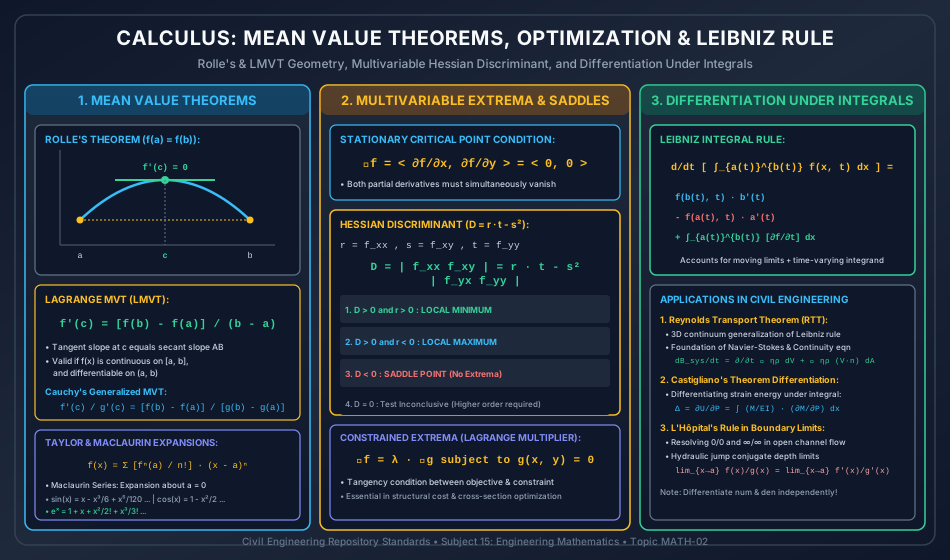
5.1 Single & Multivariable Calculus Theorems

Calculus: Mean Value Theorems, Optimization and Leibniz Rule

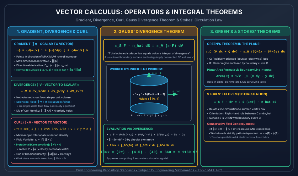
5.2 Vector Calculus Operators & Integral Theorems

Vector Calculus: Operators and Integral Theorems

6. Standard Practice Guidelines & Boundary Conditions

6.1 Requirements for Applying Integral Theorems

  1. Orientation of Boundary Curves in Green's and Stokes' Theorems:
    • The boundary curve CC must be positively oriented: traversing CC leaves the enclosed region RR or surface SS to the left (counter-clockwise in 2D).
    • In Stokes' theorem, the orientation of CC and the surface normal n^\hat{\mathbf{n}} must satisfy the right-hand rule: curling fingers along CC causes the thumb to point along n^\hat{\mathbf{n}}.
  2. Smoothness and Continuity of Vector Fields:
    • Gauss' Divergence Theorem mandates that F\mathbf{F} and its first partial derivatives are continuous throughout the closed region VV. If a point singularity exists inside VV (e.g., point source F=rr3\mathbf{F} = \frac{\mathbf{r}}{r^3} with divergence zero everywhere except at r=0r=0), VV must be punctured and an inner boundary sphere introduced.
  3. Conservative Fields and Path Independence:
    • A force field F\mathbf{F} is conservative in a simply connected domain if and only if ∇×F=0\nabla \times \mathbf{F} = \mathbf{0}.
    • The line integral ∫ABF⋅dr\int_A^B \mathbf{F} \cdot d\mathbf{r} depends solely on the endpoints AA and BB, independent of the geometric path: ∫ABF⋅dr=ϕ(B)−ϕ(A)\int_A^B \mathbf{F} \cdot d\mathbf{r} = \phi(B) - \phi(A).

7. Critical Failure Modes & Edge Cases

  1. Saddle Point Fallacy in Structural Optimization:
    • Setting ∇f=0\nabla f = \mathbf{0} yields stationary points. Assuming every critical point is a minimum leads to disastrous designs; a saddle point (D<0D < 0) has zero slope but allows uncontrolled deformation under specific load combinations.
  2. Premature Truncation of L'Hôpital's Rule:
    • If after one application of L'Hôpital's rule the quotient remains 00\frac{0}{0}, the rule must be applied repeatedly until a determinate limit emerges. Applying the rule when the form is not indeterminate (c/0c/0 or 0/c0/c) produces invalid results.
  3. Non-Simply Connected Regions (Vortex Flow Singularity):
    • For free vortex flow V=−Γ2πyx2+y2i+Γ2πxx2+y2j\mathbf{V} = -\frac{\Gamma}{2\pi}\frac{y}{x^2+y^2}\mathbf{i} + \frac{\Gamma}{2\pi}\frac{x}{x^2+y^2}\mathbf{j}: ∇×V=0for all (x,y)≠(0,0)\nabla \times \mathbf{V} = \mathbf{0} \quad \text{for all } (x, y) \neq (0, 0) However, ∮CV⋅dr=Γ≠0\oint_C \mathbf{V} \cdot d\mathbf{r} = \Gamma \neq 0 around any closed loop encircling the origin! Green's theorem cannot be applied directly across the singularity without an internal cut.

8. Worked Numerical Problems

Problem 1: Multivariable Function Critical Points, Hessian Classification & Extremum Value

Statement:
A structural potential energy landscape governing the snap-through behavior of an arched truss mechanism is expressed by:

f(x,y)=x3+y3−3xyf(x, y) = x^3 + y^3 - 3xy
  1. Find all critical points of the function f(x,y)f(x, y).
  2. Compute the second-order partial derivatives and form the Hessian discriminant D=rt−s2D = r t - s^2.
  3. Classify each critical point as a local minimum, local maximum, or saddle point.
  4. Calculate the function value at the local extremum.

Step-by-Step Analytical Solution

Part 1: Stationary Critical Points Equating first partial derivatives to zero:

∂f∂x=3x2−3y=0  ⟹  y=x2— (Eq 1)\frac{\partial f}{\partial x} = 3x^2 - 3y = 0 \implies y = x^2 \quad \text{--- (Eq 1)} ∂f∂y=3y2−3x=0  ⟹  x=y2— (Eq 2)\frac{\partial f}{\partial y} = 3y^2 - 3x = 0 \implies x = y^2 \quad \text{--- (Eq 2)}

Substituting (Eq 1) into (Eq 2):

x=(x2)2=x4  ⟹  x4−x=0  ⟹  x(x3−1)=0x = (x^2)^2 = x^4 \implies x^4 - x = 0 \implies x(x^3 - 1) = 0

Factoring:

x(x−1)(x2+x+1)=0x(x - 1)(x^2 + x + 1) = 0

Real roots:

  • x=0  ⟹  y=02=0  ⟹  P1(0,0)x = 0 \implies y = 0^2 = 0 \implies \mathbf{P_1(0, 0)}
  • x=1  ⟹  y=12=1  ⟹  P2(1,1)x = 1 \implies y = 1^2 = 1 \implies \mathbf{P_2(1, 1)}

Part 2: Second Derivatives and Discriminant

r=fxx=∂2f∂x2=6xr = f_{xx} = \frac{\partial^2 f}{\partial x^2} = 6x s=fxy=∂2f∂x∂y=−3s = f_{xy} = \frac{\partial^2 f}{\partial x \partial y} = -3 t=fyy=∂2f∂y2=6yt = f_{yy} = \frac{\partial^2 f}{\partial y^2} = 6y

The Hessian discriminant is:

D=rt−s2=(6x)(6y)−(−3)2=36xy−9D = r t - s^2 = (6x)(6y) - (-3)^2 = 36xy - 9

Part 3: Classification of Critical Points

  • At Point P1(0,0)P_1(0, 0):

    r=6(0)=0,s=−3,t=6(0)=0r = 6(0) = 0, \quad s = -3, \quad t = 6(0) = 0 D=(0)(0)−(−3)2=−9.00<0D = (0)(0) - (-3)^2 = \mathbf{-9.00 < 0}

    Since D<0D < 0, P1(0,0)P_1(0, 0) is a SADDLE POINT (No local extremum).

  • At Point P2(1,1)P_2(1, 1):

    r=6(1)=6.00>0,s=−3,t=6(1)=6.00r = 6(1) = \mathbf{6.00 > 0}, \quad s = -3, \quad t = 6(1) = 6.00 D=(6)(6)−(−3)2=36−9=27.00>0D = (6)(6) - (-3)^2 = 36 - 9 = \mathbf{27.00 > 0}

    Since D>0D > 0 and r>0r > 0, P2(1,1)P_2(1, 1) is a LOCAL MINIMUM.

Part 4: Minimum Function Value

fmin⁡=f(1,1)=(1)3+(1)3−3(1)(1)=1+1−3=−1.00f_{\min} = f(1, 1) = (1)^3 + (1)^3 - 3(1)(1) = 1 + 1 - 3 = \mathbf{-1.00}

Problem 2: Gradient, Maximum Rate of Increase, Directional Derivative & Surface Normal

Statement:
The steady-state piezometric groundwater head ϕ(x,y,z)\phi(x, y, z) in an unconfined anisotropic aquifer is described by the scalar field:

ϕ(x,y,z)=2x2y−yz2+3z(meters)\phi(x, y, z) = 2x^2 y - y z^2 + 3z \quad (\text{meters})

At the monitoring piezometer location P(1,−2,1)P(1, -2, 1):

  1. Determine the gradient vector ∇ϕ\nabla \phi.
  2. Calculate the maximum rate of spatial increase of hydraulic head and its direction.
  3. Determine the directional derivative of ϕ\phi in the direction of vector A=2i−2j+k\mathbf{A} = 2\mathbf{i} - 2\mathbf{j} + \mathbf{k}.
  4. Find the unit outward normal vector n^\hat{\mathbf{n}} to the equipotential surface passing through PP.

Step-by-Step Analytical Solution

Part 1: Gradient Vector at P(1,−2,1)P(1, -2, 1) Computing partial derivatives:

∂ϕ∂x=4xy  ⟹  ∂ϕ∂x∣P=4(1)(−2)=−8.00\frac{\partial \phi}{\partial x} = 4xy \implies \left.\frac{\partial \phi}{\partial x}\right|_P = 4(1)(-2) = \mathbf{-8.00} ∂ϕ∂y=2x2−z2  ⟹  ∂ϕ∂y∣P=2(1)2−(1)2=2−1=1.00\frac{\partial \phi}{\partial y} = 2x^2 - z^2 \implies \left.\frac{\partial \phi}{\partial y}\right|_P = 2(1)^2 - (1)^2 = 2 - 1 = \mathbf{1.00} ∂ϕ∂z=−2yz+3  ⟹  ∂ϕ∂z∣P=−2(−2)(1)+3=4+3=7.00\frac{\partial \phi}{\partial z} = -2yz + 3 \implies \left.\frac{\partial \phi}{\partial z}\right|_P = -2(-2)(1) + 3 = 4 + 3 = \mathbf{7.00}

The gradient vector is:

∇ϕ=−8.00i+1.00j+7.00k\nabla \phi = \mathbf{-8.00\mathbf{i} + 1.00\mathbf{j} + 7.00\mathbf{k}}

Part 2: Maximum Rate of Increase The maximum rate of increase occurs precisely along the gradient vector:

∣∇ϕ∣=(−8.00)2+(1.00)2+(7.00)2=64+1+49=114=10.6771 m/m|\nabla \phi| = \sqrt{(-8.00)^2 + (1.00)^2 + (7.00)^2} = \sqrt{64 + 1 + 49} = \sqrt{114} = \mathbf{10.6771\text{ m/m}}

Part 3: Directional Derivative along A=2i−2j+k\mathbf{A} = 2\mathbf{i} - 2\mathbf{j} + \mathbf{k} Magnitude of vector A\mathbf{A}:

∣A∣=22+(−2)2+12=4+4+1=9=3.00|\mathbf{A}| = \sqrt{2^2 + (-2)^2 + 1^2} = \sqrt{4 + 4 + 1} = \sqrt{9} = 3.00

Unit direction vector:

u^=A∣A∣=23i−23j+13k\hat{\mathbf{u}} = \frac{\mathbf{A}}{|\mathbf{A}|} = \frac{2}{3}\mathbf{i} - \frac{2}{3}\mathbf{j} + \frac{1}{3}\mathbf{k}

The directional derivative is the scalar dot product:

Duϕ=∇ϕ⋅u^=(−8.00)(23)+(1.00)(−23)+(7.00)(13)D_{\mathbf{u}}\phi = \nabla \phi \cdot \hat{\mathbf{u}} = (-8.00)\left(\frac{2}{3}\right) + (1.00)\left(-\frac{2}{3}\right) + (7.00)\left(\frac{1}{3}\right) Duϕ=−16.00−2.00+7.003=−11.003=−3.6667 m/mD_{\mathbf{u}}\phi = \frac{-16.00 - 2.00 + 7.00}{3} = \frac{-11.00}{3} = \mathbf{-3.6667\text{ m/m}}

Part 4: Unit Normal to Level Surface The unit normal to the equipotential surface ϕ=const\phi = \text{const} is:

n^=∇ϕ∣∇ϕ∣=−8i+j+7k114=−0.7493i+0.0937j+0.6556k\hat{\mathbf{n}} = \frac{\nabla \phi}{|\nabla \phi|} = \frac{-8\mathbf{i} + \mathbf{j} + 7\mathbf{k}}{\sqrt{114}} = \mathbf{-0.7493\mathbf{i} + 0.0937\mathbf{j} + 0.6556\mathbf{k}}

Problem 3: Gauss' Divergence Theorem Surface Flux Verification

Statement:
A convective pollutant flux density in an urban airshed is represented by the 3D vector field:

F=4xzi−y2j+yzk(kg/(m2⋅s))\mathbf{F} = 4xz \mathbf{i} - y^2 \mathbf{j} + yz \mathbf{k} \quad (\text{kg}/(\text{m}^2\cdot\text{s}))

Evaluate the total outward mass flux Φ=∬SF⋅n^dS\Phi = \iint_S \mathbf{F} \cdot \hat{\mathbf{n}} dS emerging through the closed surface SS of a cylindrical control volume bounded by:

x2+y2=9.00(R=3.00 m),z=0.00 m,andz=4.00 mx^2 + y^2 = 9.00 \quad (R = 3.00\text{ m}), \quad z = 0.00\text{ m}, \quad \text{and} \quad z = 4.00\text{ m}

Step-by-Step Analytical Solution

By Gauss' Divergence Theorem:

∬SF⋅n^dS=∭V(∇⋅F)dV\iint_S \mathbf{F} \cdot \hat{\mathbf{n}} dS = \iiint_V (\nabla \cdot \mathbf{F}) dV

Step 1: Compute the Divergence of F\mathbf{F}

∇⋅F=∂∂x(4xz)+∂∂y(−y2)+∂∂z(yz)\nabla \cdot \mathbf{F} = \frac{\partial}{\partial x}(4xz) + \frac{\partial}{\partial y}(-y^2) + \frac{\partial}{\partial z}(yz) ∇⋅F=4z−2y+z=5z−2y\nabla \cdot \mathbf{F} = 4z - 2y + z = \mathbf{5z - 2y}

Step 2: Transform to Cylindrical Coordinates In cylindrical coordinates:

x=rcos⁡θ,y=rsin⁡θ,z=zx = r \cos\theta, \quad y = r \sin\theta, \quad z = z

Volume element: dV=rdrdθdzdV = r dr d\theta dz. Limits of integration:

  • Radius: r∈[0.00,3.00]r \in [0.00, 3.00]
  • Azimuth: θ∈[0.00,2π]\theta \in [0.00, 2\pi]
  • Elevation: z∈[0.00,4.00]z \in [0.00, 4.00]

The volume integral becomes:

∭V(∇⋅F)dV=∫02π∫03∫04(5z−2rsin⁡θ)⋅r dz dr dθ\iiint_V (\nabla \cdot \mathbf{F}) dV = \int_{0}^{2\pi} \int_{0}^{3} \int_{0}^{4} (5z - 2r \sin\theta) \cdot r \, dz \, dr \, d\theta

Split into two integrals:

I1=∫02πdθ∫03rdr∫045zdzI_1 = \int_{0}^{2\pi} d\theta \int_{0}^{3} r dr \int_{0}^{4} 5z dz I2=∫02πsin⁡θdθ∫032r2dr∫04dzI_2 = \int_{0}^{2\pi} \sin\theta d\theta \int_{0}^{3} 2r^2 dr \int_{0}^{4} dz

Step 3: Evaluate Integrals For I2I_2:

∫02πsin⁡θdθ=[−cos⁡θ]02π=−1−(−1)=0  ⟹  I2=0.00\int_{0}^{2\pi} \sin\theta d\theta = [-\cos\theta]_0^{2\pi} = -1 - (-1) = 0 \implies \mathbf{I_2 = 0.00}

(Due to geometric symmetry, the net convective flux from the −2y-2y term identically cancels out across the cylinder).

For I1I_1:

∫02πdθ=2π\int_{0}^{2\pi} d\theta = 2\pi ∫03rdr=[r22]03=92=4.50\int_{0}^{3} r dr = \left[\frac{r^2}{2}\right]_0^3 = \frac{9}{2} = 4.50 ∫045zdz=[5z22]04=5(16)2=40.00\int_{0}^{4} 5z dz = \left[\frac{5z^2}{2}\right]_0^4 = \frac{5(16)}{2} = 40.00

Multiplying:

I1=(2π)×(4.50)×(40.00)=(9π)×(40.00)=360πI_1 = (2\pi) \times (4.50) \times (40.00) = (9\pi) \times (40.00) = \mathbf{360\pi} Φ=360π≈1130.9734 kg/s(1130.97 kg/s)\Phi = 360\pi \approx \mathbf{1130.9734\text{ kg/s}} \quad (1130.97\text{ kg/s})

9. Comparative Exam Analysis

Parameter / Feature GATE CE UPSC ESE (Paper 1 & GS) SSC JE & State AE RRB JE
Typical Question Formats High-precision numericals: Directional derivative, Gauss flux, Lagrange MVT cc value Analytical & Concept: Condition for solenoidal/irrotational, Green's area formula Direct MCQs: Definition of gradient, condition for Rolle's theorem, L'Hôpital forms Elementary limits: Simple derivatives, basic integration formulas
Primary Focus Areas Vector calculus theorems (Gauss, Stokes, Green), maxima/minima discriminant DD Line integrals, conservative work done ∮F⋅dr=0\oint \mathbf{F}\cdot d\mathbf{r} = 0, Leibniz differentiation ∇⋅V=0\nabla \cdot \mathbf{V} = 0, ∇×V=0\nabla \times \mathbf{V} = \mathbf{0}, critical points fx=fy=0f_x=f_y=0 Standard limits (lim⁡x→0sin⁡xx=1\lim_{x\to 0}\frac{\sin x}{x}=1), power rule, exponential derivatives
Scoring Traps Forgetting to divide by ∣A∣|\mathbf{A}| for directional derivative; using D<0D < 0 as extremum Neglecting boundary orientation in Green's theorem; dividing by cc in Cauchy MVT Confusing solenoidal (div=0\text{div}=0) with irrotational (curl=0\text{curl}=0) Claiming Rolle's theorem holds when f(a)≠f(b)f(a) \neq f(b)

10. Common Pitfalls & Traps

  1. Directional Derivative Unit Vector Omission:
    • Trap: Computing DAϕ=∇ϕ⋅AD_{\mathbf{A}}\phi = \nabla \phi \cdot \mathbf{A}.
    • Correction: The directional derivative requires the unit vector u^=A∣A∣\hat{\mathbf{u}} = \frac{\mathbf{A}}{|\mathbf{A}|}. Omitting normalization scales the derivative by ∣A∣|\mathbf{A}|.
  2. Saddle Point Identification (D<0D < 0):
    • Trap: If D=rt−s2<0D = r t - s^2 < 0, checking whether r>0r > 0 or r<0r < 0 to declare a minimum or maximum.
    • Correction: If D<0D < 0, the critical point is always a saddle point, regardless of the sign of rr! The sign of rr is only tested when D>0D > 0.
  3. Leibniz Rule Moving Limits:
    • Trap: Forgetting to multiply by the boundary derivatives b′(t)b'(t) and a′(t)a'(t).
    • Correction: The boundary contribution is f(b(t),t)b′(t)−f(a(t),t)a′(t)f(b(t), t)b'(t) - f(a(t), t)a'(t). If limits are fixed constants, these terms naturally drop to zero.
  4. Surface Orientation in Stokes' Theorem:
    • Trap: Integrating curl without matching the surface normal n^\hat{\mathbf{n}} to the loop circulation via the right-hand rule.
    • Correction: Reversing n^\hat{\mathbf{n}} introduces an erroneous negative sign into the circulation.

11. Real-World Civil & Structural Applications

  1. Fluid Mechanics & Hydraulic Modeling (Continuity & Navier-Stokes):
    • The continuity equation ∂ρ∂t+∇⋅(ρV)=0\frac{\partial \rho}{\partial t} + \nabla \cdot (\rho \mathbf{V}) = 0 is the direct physical manifestation of Gauss' Divergence Theorem applied to fluid mass conservation. For water (ρ=const\rho = \text{const}), ∇⋅V=0\nabla \cdot \mathbf{V} = 0.
  2. Groundwater Seepage & Flow Nets (Laplace Equation):
    • In Darcy flow through porous soil media, velocity v=−k∇h\mathbf{v} = -k \nabla h. Substituting into continuity ∇⋅v=0\nabla \cdot \mathbf{v} = 0 yields the 2D Laplace equation ∇2h=∂2h∂x2+∂2h∂z2=0\nabla^2 h = \frac{\partial^2 h}{\partial x^2} + \frac{\partial^2 h}{\partial z^2} = 0, forming orthogonal equipotential and streamlines.
  3. Automated Earthwork & GIS Topographic Contouring:
    • Digital elevation models (DEMs) use gradient vectors ∇z(x,y)\nabla z(x, y) to compute steepest slope run-off paths, delineate watershed basin divides, and calculate cut-and-fill earthwork volumes.

12. Comprehensive Summary & Quick Revision Guide

  • LMVT: f′(c)=f(b)−f(a)b−af'(c) = \frac{f(b) - f(a)}{b - a} for c∈(a,b)c \in (a, b).
  • Rolle's: If f(a)=f(b)  ⟹  f′(c)=0f(a) = f(b) \implies f'(c) = 0.
  • Hessian Discriminant: D=rt−s2=fxxfyy−(fxy)2D = r t - s^2 = f_{xx}f_{yy} - (f_{xy})^2.
    • D>0,r>0  ⟹  D > 0, r > 0 \implies Local Minimum.
    • D>0,r<0  ⟹  D > 0, r < 0 \implies Local Maximum.
    • D<0  ⟹  D < 0 \implies Saddle Point.
  • Gradient: ∇ϕ\nabla \phi gives direction and magnitude of maximum rate of increase. Directional derivative Duϕ=∇ϕ⋅u^D_{\mathbf{u}}\phi = \nabla \phi \cdot \hat{\mathbf{u}}. Surface normal n^=∇ϕ/∣∇ϕ∣\hat{\mathbf{n}} = \nabla \phi / |\nabla \phi|.
  • Divergence: ∇⋅V\nabla \cdot \mathbf{V}. Solenoidal if ∇⋅V=0\nabla \cdot \mathbf{V} = 0.
  • Curl: ∇×V\nabla \times \mathbf{V}. Irrotational / Conservative if ∇×V=0  ⟹  V=∇ϕ\nabla \times \mathbf{V} = \mathbf{0} \implies \mathbf{V} = \nabla \phi.
  • Identities: ∇×(∇ϕ)=0\nabla \times (\nabla \phi) = \mathbf{0}, ∇⋅(∇×A)=0\nabla \cdot (\nabla \times \mathbf{A}) = 0.
  • Gauss Theorem: ∬SF⋅n^dS=∭V(∇⋅F)dV\iint_S \mathbf{F} \cdot \hat{\mathbf{n}} dS = \iiint_V (\nabla \cdot \mathbf{F}) dV.
  • Green's Theorem: ∮C(Pdx+Qdy)=∬R(∂Q∂x−∂P∂y)dA\oint_C (P dx + Q dy) = \iint_R (\frac{\partial Q}{\partial x} - \frac{\partial P}{\partial y}) dA. Area =12∮C(xdy−ydx)= \frac{1}{2}\oint_C (x dy - y dx).
  • Stokes' Theorem: ∮CF⋅dr=∬S(∇×F)⋅n^dS\oint_C \mathbf{F} \cdot d\mathbf{r} = \iint_S (\nabla \times \mathbf{F}) \cdot \hat{\mathbf{n}} dS.

13. Practice Problems for Self-Assessment

  1. LMVT Practice: Find the value of cc guaranteed by Lagrange's MVT for f(x)=x2−4x+3f(x) = x^2 - 4x + 3 on the interval [1,4][1, 4].
    (Answer: f(1)=0,f(4)=3  ⟹  f(4)−f(1)4−1=3−03=1f(1) = 0, f(4) = 3 \implies \frac{f(4) - f(1)}{4 - 1} = \frac{3 - 0}{3} = 1. f′(c)=2c−4=1  ⟹  2c=5  ⟹  c=2.50∈(1,4)f'(c) = 2c - 4 = 1 \implies 2c = 5 \implies c = \mathbf{2.50} \in (1, 4))
  2. Solenoidal Vector Practice: Find constant aa such that vector field V=(x+3y)i+(y−2z)j+(x+az)k\mathbf{V} = (x + 3y)\mathbf{i} + (y - 2z)\mathbf{j} + (x + a z)\mathbf{k} is solenoidal.
    (Answer: ∇⋅V=∂∂x(x+3y)+∂∂y(y−2z)+∂∂z(x+az)=1+1+a=2+a=0  ⟹  a=−2.00\nabla \cdot \mathbf{V} = \frac{\partial}{\partial x}(x+3y) + \frac{\partial}{\partial y}(y-2z) + \frac{\partial}{\partial z}(x+az) = 1 + 1 + a = 2 + a = 0 \implies a = \mathbf{-2.00})
  3. Conservative Work Practice: Verify that F=(2xy+z3)i+x2j+3xz2k\mathbf{F} = (2xy + z^3)\mathbf{i} + x^2 \mathbf{j} + 3xz^2 \mathbf{k} is conservative, and calculate the work done moving a particle from (1,−2,1)(1, -2, 1) to (3,1,4)(3, 1, 4).
    (Answer: ∇×F=0\nabla \times \mathbf{F} = \mathbf{0}; Potential function ϕ=x2y+xz3\phi = x^2 y + x z^3. Work W=ϕ(3,1,4)−ϕ(1,−2,1)=[32(1)+3(43)]−[12(−2)+1(13)]=[9+192]−[−2+1]=201−(−1)=202.00 JW = \phi(3, 1, 4) - \phi(1, -2, 1) = [3^2(1) + 3(4^3)] - [1^2(-2) + 1(1^3)] = [9 + 192] - [-2 + 1] = 201 - (-1) = \mathbf{202.00\text{ J}})

14. References & Standard Texts

  1. Erwin Kreyszig, Advanced Engineering Mathematics, 10th Edition, John Wiley & Sons, 2011.
  2. George B. Thomas and Maurice D. Weir, Thomas' Calculus: Early Transcendentals, 14th Edition, Pearson, 2018.
  3. B.S. Grewal, Higher Engineering Mathematics, 44th Edition, Khanna Publishers, 2017.
  4. James Stewart, Calculus: Early Transcendentals, 8th Edition, Cengage Learning, 2015.
  5. Murray R. Spiegel, Schaum's Outline of Vector Analysis, 2nd Edition, McGraw-Hill, 2009.