MATH-01 Chapter 01 · Linear Algebra

Linear Algebra: Matrices, Systems of Linear Equations, Rank, Eigenvalues, Eigenvectors & Structural Stiffness Applications

In this chapter (1 topics)
On this page

1. Executive Summary & Core Definitions

Linear Algebra is the fundamental mathematical language of modern computational mechanics, finite element analysis (FEA), structural matrix methods, and continuum mechanics in civil engineering. Every structural frame, soil continuum, fluid grid, and highway network discretized into nodes and elements culminates in algebraic systems of equations governing force equilibrium, kinematic compatibility, vibration modes, and stress states.

Core Terminology & Definitions

  • Matrix: A rectangular array of numbers, symbols, or expressions arranged in mm rows and nn columns (m×nm \times n).
  • Symmetric Matrix: A square matrix AA where AT=AA^T = A (aij=ajia_{ij} = a_{ji}). All real symmetric matrices have strictly real eigenvalues, and eigenvectors corresponding to distinct eigenvalues are mutually orthogonal.
  • Skew-Symmetric Matrix: A square matrix where AT=−AA^T = -A (aij=−ajia_{ij} = -a_{ji}, which implies all diagonal elements aii=0a_{ii} = 0). Its eigenvalues are purely imaginary or zero.
  • Orthogonal Matrix: A real square matrix QQ satisfying QTQ=QQT=IQ^T Q = Q Q^T = I, meaning Q−1=QTQ^{-1} = Q^T and det⁡(Q)=±1\det(Q) = \pm 1. Represents rigid-body rotations and reflections.
  • Rank of a Matrix (rank(A)\text{rank}(A) or ρ(A)\rho(A)): The maximum number of linearly independent row vectors (or column vectors) in AA, or the order of the highest-order non-zero determinant minor.
  • Nullity (nullity(A)\text{nullity}(A)): The dimension of the null space (kernel) of AA, representing the number of linearly independent solutions to the homogeneous equation Ax=0A\mathbf{x} = \mathbf{0}.
  • Consistent System: A linear system Ax=bA\mathbf{x} = \mathbf{b} possessing at least one solution (either a unique solution or infinitely many solutions).
  • Eigenvalue (λ\lambda): A scalar multiplier such that linear transformation by AA merely scales the non-zero vector v\mathbf{v} without altering its direction: Av=λvA\mathbf{v} = \lambda \mathbf{v}.
  • Eigenvector (v\mathbf{v}): A non-zero vector whose direction remains unchanged under the linear transformation represented by AA.
  • Characteristic Equation: The polynomial equation det⁡(A−λI)=0\det(A - \lambda I) = 0 whose roots are the eigenvalues of AA.
  • Cayley-Hamilton Theorem: The theorem asserting that every square matrix satisfies its own characteristic algebraic equation: P(A)=[0]P(A) = [0].
  • Stiffness Matrix ([K][K]): In structural engineering, a square matrix relating generalized nodal displacements {Δ}\{\Delta\} to generalized nodal forces {P}\{P\}: {P}=[K]{Δ}\{P\} = [K]\{\Delta\}. It is inherently symmetric (Betti's reciprocal theorem) and positive-definite for stable, constrained structures.

2. Foundational Principles & Governing Axioms

2.1 Matrix Operations & Determinant Theorems

  1. Determinant Properties:
    • det⁡(AT)=det⁡(A)\det(A^T) = \det(A).
    • det⁡(AB)=det⁡(A)⋅det⁡(B)\det(A B) = \det(A) \cdot \det(B) (for square matrices of identical size).
    • det⁡(kA)=kndet⁡(A)\det(k A) = k^n \det(A) for an n×nn \times n matrix.
    • det⁡(A−1)=1det⁡(A)\det(A^{-1}) = \frac{1}{\det(A)} (provided AA is non-singular, det⁡(A)≠0\det(A) \neq 0).
    • Interchanging any two rows (or columns) reverses the sign of the determinant: det⁡(A′)=−det⁡(A)\det(A') = -\det(A).
    • If two rows (or columns) are identical or proportional, det⁡(A)=0\det(A) = 0.
    • Adding a scalar multiple of one row to another row leaves the determinant strictly unchanged: det⁡(A′)=det⁡(A)\det(A') = \det(A).
  2. Matrix Inverse (A−1A^{-1}): A−1=adj(A)det⁡(A)A^{-1} = \frac{\text{adj}(A)}{\det(A)} where adj(A)=[Cij]T\text{adj}(A) = [C_{ij}]^T is the adjugate matrix (transpose of the cofactor matrix Cij=(−1)i+jMijC_{ij} = (-1)^{i+j} M_{ij}).
    • (AB)−1=B−1A−1(A B)^{-1} = B^{-1} A^{-1} (Reversal rule for inverses).
    • (AT)−1=(A−1)T(A^T)^{-1} = (A^{-1})^T.

2.2 Row Echelon Forms & Gaussian Elimination

By applying elementary row operations:

  1. Ri↔RjR_i \leftrightarrow R_j (Row interchange)
  2. Ri←kRiR_i \leftarrow k R_i (k≠0k \neq 0, Row scaling)
  3. Ri←Ri+cRjR_i \leftarrow R_i + c R_j (Row addition)

Any matrix can be reduced to Row Echelon Form (REF):

  • All non-zero rows are strictly above all zero rows.
  • The leading entry (pivot) of each non-zero row is strictly to the right of the leading entry of the row above it.
  • All entries below a leading pivot are zero.

Reduced Row Echelon Form (RREF) / Gauss-Jordan Form:

  • Each leading entry is normalized to 11.
  • Each leading 11 is the only non-zero entry in its column (entries both below and above are zero).

The Rank of AA:

rank(A)=Number of non-zero rows (pivots) in its REF or RREF\text{rank}(A) = \text{Number of non-zero rows (pivots) in its REF or RREF}

2.3 The Rouché-Capelli Theorem for Systems of Linear Equations

For a system of mm linear equations in nn unknowns:

Ax=b  ⟺  [a11a12…a1na21a22…a2n⋮⋮⋱⋮am1am2…amn]{x1x2⋮xn}={b1b2⋮bm}A \mathbf{x} = \mathbf{b} \iff \begin{bmatrix} a_{11} & a_{12} & \dots & a_{1n} \\ a_{21} & a_{22} & \dots & a_{2n} \\ \vdots & \vdots & \ddots & \vdots \\ a_{m1} & a_{m2} & \dots & a_{mn} \end{bmatrix} \begin{Bmatrix} x_1 \\ x_2 \\ \vdots \\ x_n \end{Bmatrix} = \begin{Bmatrix} b_1 \\ b_2 \\ \vdots \\ b_m \end{Bmatrix}

Form the augmented matrix [A∣b][A | \mathbf{b}] of size m×(n+1)m \times (n+1).

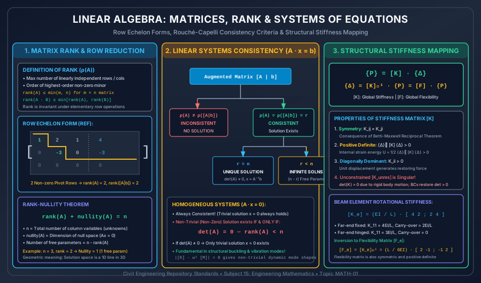
                            Augmented Matrix [A | b]
                                       │
                 ┌─────────────────────┴─────────────────────┐
                 │                                           │
       rank(A) ≠ rank([A|b])                       rank(A) = rank([A|b]) = r
                 │                                           │
           INCONSISTENT                                  CONSISTENT
          (No Solution)                               (Solution Exists)
                                                             │
                                     ┌───────────────────────┴───────────────────────┐
                                     │                                               │
                                   r = n                                           r < n
                                     │                                               │
                              UNIQUE SOLUTION                                INFINITE SOLUTIONS
                              (det(A) ≠ 0)                                 (n - r Free Parameters)
  1. Non-Homogeneous Systems (Ax=bA\mathbf{x} = \mathbf{b}, with b≠0\mathbf{b} \neq \mathbf{0}):
    • Case 1 (Inconsistent): rank(A)≠rank([A∣b])\text{rank}(A) \neq \text{rank}([A|\mathbf{b}]). The system has NO SOLUTION. (Occurs when row reduction yields a contradictory row [00…0∣c]\begin{bmatrix} 0 & 0 & \dots & 0 & | & c \end{bmatrix} with c≠0c \neq 0).
    • Case 2 (Unique Solution): rank(A)=rank([A∣b])=n\text{rank}(A) = \text{rank}([A|\mathbf{b}]) = n (where nn is the number of unknowns). For a square system (n×nn \times n), this occurs if and only if det⁡(A)≠0\det(A) \neq 0. Solution: x=A−1b\mathbf{x} = A^{-1}\mathbf{b}.
    • Case 3 (Infinitely Many Solutions): rank(A)=rank([A∣b])=r<n\text{rank}(A) = \text{rank}([A|\mathbf{b}]) = r < n. The general solution contains (n−r)(n - r) linearly independent arbitrary parameters.
  2. Homogeneous Systems (Ax=0A\mathbf{x} = \mathbf{0}):
    • The augmented matrix [A∣0][A|\mathbf{0}] always has rank(A)=rank([A∣0])\text{rank}(A) = \text{rank}([A|\mathbf{0}]). Therefore, homogeneous systems are always consistent.
    • The trivial solution x=0\mathbf{x} = \mathbf{0} always exists.
    • A non-trivial (non-zero) solution exists if and only if rank(A)<n\text{rank}(A) < n, which for a square matrix (n×nn \times n) means det⁡(A)=0\det(A) = 0.

3. Step-by-Step Analytical Derivations

3.1 The Rank-Nullity Theorem

Let T:Rn→RmT: \mathbb{R}^n \to \mathbb{R}^m be a linear transformation represented by m×nm \times n matrix AA. The kernel (null space) is:

Null(A)={x∈Rn:Ax=0}\text{Null}(A) = \{\mathbf{x} \in \mathbb{R}^n : A\mathbf{x} = \mathbf{0}\}

The range (column space) is:

Col(A)={y∈Rm:y=Ax for some x∈Rn}\text{Col}(A) = \{\mathbf{y} \in \mathbb{R}^m : \mathbf{y} = A\mathbf{x} \text{ for some } \mathbf{x} \in \mathbb{R}^n\}

By row-reducing AA to RREF:

  • The columns containing pivots correspond to linearly independent column vectors forming a basis for Col(A)\text{Col}(A). The number of pivots is r=rank(A)r = \text{rank}(A).
  • The remaining columns without pivots correspond to free variables. Expressing the basic variables in terms of the free variables yields (n−r)(n - r) linearly independent basis vectors spanning Null(A)\text{Null}(A). Therefore:
nullity(A)=dim⁡(Null(A))=n−r=n−rank(A)\text{nullity}(A) = \dim(\text{Null}(A)) = n - r = n - \text{rank}(A) rank(A)+nullity(A)=n\text{rank}(A) + \text{nullity}(A) = n

3.2 Spectral Invariants of Eigenvalues

Let AA be an n×nn \times n matrix with eigenvalues λ1,λ2,…,λn\lambda_1, \lambda_2, \dots, \lambda_n. The characteristic polynomial is:

P(λ)=det⁡(A−λI)=(−1)nλn+(−1)n−1cn−1λn−1+⋯+c1λ+c0P(\lambda) = \det(A - \lambda I) = (-1)^n \lambda^n + (-1)^{n-1} c_{n-1} \lambda^{n-1} + \dots + c_1 \lambda + c_0

Factoring by roots:

P(λ)=(λ1−λ)(λ2−λ)…(λn−λ)P(\lambda) = (\lambda_1 - \lambda)(\lambda_2 - \lambda) \dots (\lambda_n - \lambda)
  1. Sum of Eigenvalues (Trace Invariant): Comparing the coefficient of (−λ)n−1(-\lambda)^{n-1}: cn−1=∑i=1naii=Tr(A)c_{n-1} = \sum_{i=1}^n a_{ii} = \text{Tr}(A) From the factored form, the sum of roots is: ∑i=1nλi=Tr(A)\sum_{i=1}^n \lambda_i = \text{Tr}(A)
  2. Product of Eigenvalues (Determinant Invariant): Evaluating P(λ)P(\lambda) at λ=0\lambda = 0: P(0)=det⁡(A−0⋅I)=det⁡(A)P(0) = \det(A - 0 \cdot I) = \det(A) From the factored form: P(0)=λ1⋅λ2…λn=∏i=1nλiP(0) = \lambda_1 \cdot \lambda_2 \dots \lambda_n = \prod_{i=1}^n \lambda_i ∏i=1nλi=det⁡(A)\prod_{i=1}^n \lambda_i = \det(A)

3.3 Analytical Derivation of Cayley-Hamilton Applications

The Cayley-Hamilton Theorem states:

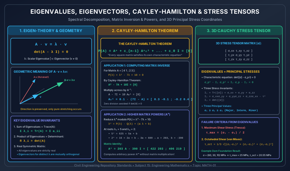
P(A)=An−Tr(A)An−1+⋯+(−1)ndet⁡(A)I=[0]P(A) = A^n - \text{Tr}(A) A^{n-1} + \dots + (-1)^n \det(A) I = [0]

Matrix Inversion via Cayley-Hamilton:

For an n×nn \times n invertible matrix with det⁡(A)≠0\det(A) \neq 0:

(−1)n−1det⁡(A)I=An+cn−1An−1+⋯+c1A(-1)^{n-1} \det(A) I = A^n + c_{n-1} A^{n-1} + \dots + c_1 A

Multiplying both sides by A−1A^{-1}:

(−1)n−1det⁡(A)A−1=An−1+cn−1An−2+⋯+c1I(-1)^{n-1} \det(A) A^{-1} = A^{n-1} + c_{n-1} A^{n-2} + \dots + c_1 I A−1=(−1)ndet⁡(A)[An−1+cn−1An−2+⋯+c1I]A^{-1} = \frac{(-1)^n}{\det(A)} \left[A^{n-1} + c_{n-1} A^{n-2} + \dots + c_1 I\right]

For a 2×22 \times 2 matrix AA where P(λ)=λ2−Tr(A)λ+det⁡(A)=0P(\lambda) = \lambda^2 - \text{Tr}(A)\lambda + \det(A) = 0:

A2−Tr(A)A+det⁡(A)I=[0]  ⟹  A−1=1det⁡(A)[Tr(A)I−A]A^2 - \text{Tr}(A) A + \det(A) I = [0] \implies A^{-1} = \frac{1}{\det(A)}\left[\text{Tr}(A) I - A\right]

Computing High Matrix Powers (AmA^m):

By polynomial division, any power λm\lambda^m (where m≥nm \ge n) can be written as:

λm=P(λ)⋅Q(λ)+R(λ)\lambda^m = P(\lambda) \cdot Q(\lambda) + R(\lambda)

where the remainder R(λ)=an−1λn−1+⋯+a1λ+a0R(\lambda) = a_{n-1} \lambda^{n-1} + \dots + a_1 \lambda + a_0 has degree <n< n. Evaluating at the nn distinct eigenvalues λi\lambda_i:

λim=R(λi)\lambda_i^m = R(\lambda_i)

Solving this n×nn \times n Vandermonde linear system yields coefficients a0,…,an−1a_0, \dots, a_{n-1}. Substituting matrix AA (since P(A)=[0]P(A) = [0]):

Am=an−1An−1+⋯+a1A+a0IA^m = a_{n-1} A^{n-1} + \dots + a_1 A + a_0 I

3.4 3D Cauchy Stress Tensor Spectral Decomposition

In continuum mechanics, the stress state at a point is represented by the second-order symmetric Cauchy stress tensor [σ][\sigma]:

[σ]=[σxxτxyτxzτyxσyyτyzτzxτzyσzz][\sigma] = \begin{bmatrix} \sigma_{xx} & \tau_{xy} & \tau_{xz} \\ \tau_{yx} & \sigma_{yy} & \tau_{yz} \\ \tau_{zx} & \tau_{zy} & \sigma_{zz} \end{bmatrix}

A plane with unit normal n=[nx,ny,nz]T\mathbf{n} = [n_x, n_y, n_z]^T is a principal plane if the traction vector T(n)=[σ]n\mathbf{T}^{(\mathbf{n})} = [\sigma] \mathbf{n} acts purely normal to the plane with zero shear:

[σ]n=σpn  ⟺  ([σ]−σpI)n=0[\sigma] \mathbf{n} = \sigma_p \mathbf{n} \iff ([\sigma] - \sigma_p I) \mathbf{n} = \mathbf{0}

This is the standard eigenvalue problem. Non-trivial direction vectors n≠0\mathbf{n} \neq \mathbf{0} exist if:

det⁡([σ]−σpI)=0\det([\sigma] - \sigma_p I) = 0

Expanding the determinant yields the Cubic Stress Characteristic Equation:

σp3−I1σp2+I2σp−I3=0\sigma_p^3 - I_1 \sigma_p^2 + I_2 \sigma_p - I_3 = 0

Where the Three Stress Invariants are:

  1. First Stress Invariant (I1I_1): I1=Tr([σ])=σxx+σyy+σzz=σ1+σ2+σ3I_1 = \text{Tr}([\sigma]) = \sigma_{xx} + \sigma_{yy} + \sigma_{zz} = \sigma_1 + \sigma_2 + \sigma_3
  2. Second Stress Invariant (I2I_2): I2=∣σxxτxyτxyσyy∣+∣σyyτyzτyzσzz∣+∣σxxτxzτxzσzz∣=σ1σ2+σ2σ3+σ3σ1I_2 = \begin{vmatrix} \sigma_{xx} & \tau_{xy} \\ \tau_{xy} & \sigma_{yy} \end{vmatrix} + \begin{vmatrix} \sigma_{yy} & \tau_{yz} \\ \tau_{yz} & \sigma_{zz} \end{vmatrix} + \begin{vmatrix} \sigma_{xx} & \tau_{xz} \\ \tau_{xz} & \sigma_{zz} \end{vmatrix} = \sigma_1 \sigma_2 + \sigma_2 \sigma_3 + \sigma_3 \sigma_1
  3. Third Stress Invariant (I3I_3): I3=det⁡([σ])=σ1σ2σ3I_3 = \det([\sigma]) = \sigma_1 \sigma_2 \sigma_3

The three ordered real roots σ1≥σ2≥σ3\sigma_1 \ge \sigma_2 \ge \sigma_3 are the Major, Intermediate, and Minor Principal Stresses.

  • Maximum Shear Stress (Tresca Yield Criterion): τmax⁡=σ1−σ32\tau_{\max} = \frac{\sigma_1 - \sigma_3}{2}
  • Octahedral Shear Stress (von Mises Yield Criterion): τoct=13(σ1−σ2)2+(σ2−σ3)2+(σ3−σ1)2=23J2\tau_{\text{oct}} = \frac{1}{3} \sqrt{(\sigma_1 - \sigma_2)^2 + (\sigma_2 - \sigma_3)^2 + (\sigma_3 - \sigma_1)^2} = \sqrt{\frac{2}{3} J_2}

4. Key Formulas & Summary Tables

4.1 Master Formula Table

Mathematical Concept Governing Equation Significance / Engineering Application
Rank-Nullity Theorem rank(A)+nullity(A)=n\text{rank}(A) + \text{nullity}(A) = n Relates independent equations, unknowns, and degree of indeterminacy
Consistency Condition rank(A)=rank([A∥b])\text{rank}(A) = \text{rank}([A\|\mathbf{b}]) Condition for existence of solutions to Ax=bA\mathbf{x} = \mathbf{b}
Unique Solution rank(A)=rank([A∥b])=n\text{rank}(A) = \text{rank}([A\|\mathbf{b}]) = n Square system has det⁡(A)≠0\det(A) \neq 0; x=A−1b\mathbf{x} = A^{-1}\mathbf{b}
Infinite Solutions rank(A)=rank([A∥b])=r<n\text{rank}(A) = \text{rank}([A\|\mathbf{b}]) = r < n Number of free parameters = n−rn - r
Homogeneous System Ax=0  ⟹  det⁡(A)=0A\mathbf{x} = \mathbf{0} \implies \det(A) = 0 Condition for non-trivial vibration mode / buckling load
Trace Invariant ∑i=1nλi=Tr(A)=∑aii\sum_{i=1}^n \lambda_i = \text{Tr}(A) = \sum a_{ii} Sum of eigenvalues equals sum of main diagonal entries
Determinant Invariant ∏i=1nλi=det⁡(A)\prod_{i=1}^n \lambda_i = \det(A) Product of eigenvalues equals matrix determinant
Cayley-Hamilton P(A)=[0]P(A) = [0] Enables matrix inversion and higher power evaluations
Maximum Shear Stress τmax⁡=σ1−σ32\tau_{\max} = \frac{\sigma_1 - \sigma_3}{2} Critical Tresca shear failure in soils, concrete, and metals
Octahedral Shear τoct=13∑(σi−σj)2\tau_{\text{oct}} = \frac{1}{3}\sqrt{\sum (\sigma_i - \sigma_j)^2} von Mises equivalent stress criterion in structural steel

4.2 Special Matrix Types in Civil Engineering

Matrix Type Mathematical Definition Key Property Civil / Structural Example
Symmetric AT=AA^T = A Real eigenvalues; orthogonal eigenvectors Structural stiffness matrix [K][K], stress tensor [σ][\sigma]
Positive Definite xTAx>0  (∀x≠0)\mathbf{x}^T A \mathbf{x} > 0 \; (\forall \mathbf{x} \neq \mathbf{0}) All λi>0\lambda_i > 0, det⁡(A)>0\det(A) > 0, unique minimum strain energy Constrained structural stiffness [K][K], mass matrix [M][M]
Orthogonal QTQ=I  ⟹  Q−1=QTQ^T Q = I \implies Q^{-1} = Q^T Preserves lengths and angles; det⁡(Q)=±1\det(Q) = \pm 1 2D/3D coordinate transformation matrices [T][T] in FEA
Idempotent A2=AA^2 = A Eigenvalues are strictly 00 or 11 Projection matrices in least squares regression surveying
Diagonal D=diag(d1,…,dn)D = \text{diag}(d_1, \dots, d_n) Powers Dk=diag(d1k,…,dnk)D^k = \text{diag}(d_1^k, \dots, d_n^k), det⁡(D)=∏di\det(D) = \prod d_i Modal decoupled equations of motion in dynamics

5. Visual Architectural Diagrams

5.1 Matrix Rank, Row Reduction & Linear System Consistency

Linear Algebra: Matrices, Rank and Systems of Equations

5.2 Eigenvalues, Cayley-Hamilton & 3D Stress Tensors

Eigenvalues, Eigenvectors, Cayley-Hamilton and Stress Tensors

6. Standard Practice Guidelines & Boundary Conditions

6.1 Boundary Conditions in Finite Element Stiffness Analysis

  1. Unconstrained Global Stiffness Matrix [Kunres][K_{\text{unres}}]:
    • For an unconstrained structural assembly of NN degrees of freedom, rigid body translations and rotations can occur without inducing internal strain energy.
    • Consequently, [Kunres]vrigid=0  ⟹  det⁡([Kunres])=0[K_{\text{unres}}] \mathbf{v}_{\text{rigid}} = \mathbf{0} \implies \det([K_{\text{unres}}]) = 0.
    • The unconstrained matrix is singular and cannot be inverted!
  2. Application of Boundary Conditions (Elimination Method):
    • For every fixed degree of freedom (where displacement Δk=0\Delta_k = 0), the kk-th row and kk-th column of the global stiffness matrix are eliminated.
    • The resulting reduced stiffness matrix [Kreduced][K_{\text{reduced}}] is strictly symmetric and positive-definite (det⁡([Kreduced])>0\det([K_{\text{reduced}}]) > 0), ensuring a unique stable solution: {Δfree}=[Kreduced]−1{Papplied}\{\Delta_{\text{free}}\} = [K_{\text{reduced}}]^{-1} \{P_{\text{applied}}\}

6.2 Condition Number & Numerical Stability

In structural matrix software (SAP2000, STAAD.Pro, ANSYS), numerical accuracy is governed by the matrix Condition Number (κ\kappa):

κ(A)=∥A∥⋅∥A−1∥=λmax⁡λmin⁡\kappa(A) = \|A\| \cdot \|A^{-1}\| = \frac{\lambda_{\max}}{\lambda_{\min}}
  • If κ(A)≈1−100\kappa(A) \approx 1 - 100: Well-conditioned matrix; stable numerical inversion.
  • If κ(A)>107\kappa(A) > 10^7: Ill-conditioned matrix; small round-off errors in loads {P}\{P\} create massive errors in displacements {Δ}\{\Delta\}. Common causes include mixing extremely stiff structural elements (e.g., massive shear walls) with extremely flexible members (e.g., slender cables) in the same model.

7. Critical Failure Modes & Edge Cases

  1. Defective Matrices (Non-Diagonalizable):
    • If an eigenvalue has algebraic multiplicity m>1m > 1, but the geometric multiplicity (number of linearly independent eigenvectors) is g<mg < m, the matrix lacks a full set of basis eigenvectors.
    • It cannot be diagonalized as PDP−1P D P^{-1}; Jordan Canonical Form must be utilized.
  2. Zero Pivot during Gaussian Elimination:
    • Encountering a zero pivot on the diagonal does not imply singularity. Partial pivoting (row interchange Ri↔RjR_i \leftrightarrow R_j) is mandatory to bring the largest magnitude element to the pivot position, preventing catastrophic numerical overflow.
  3. Singular Stress Matrix in Geotechnical Stability:
    • In 2D plane strain analysis, if the stress determinant I3=0I_3 = 0, one principal stress is zero (e.g., unconfined compression). In Mohr-Coulomb failure, if σ3≤0\sigma_3 \le 0 (tensile stress in cohesionless sand), liquefaction or tensile spalling occurs.

8. Worked Numerical Problems

Problem 1: System of Linear Equations Consistency and Parametric Solution Space

Statement:
A statically indeterminate space truss joint is analyzed under external nodal equilibrium. The governing linear equations relating three member forces (x,y,zx, y, z) are:

x+2y+z=42x+y+2z=5x−y+z=1\begin{aligned} x + 2y + z &= 4 \\ 2x + y + 2z &= 5 \\ x - y + z &= 1 \end{aligned}

Using Gaussian elimination and the Rouché-Capelli theorem:

  1. Form the augmented matrix [A∣b][A | \mathbf{b}] and reduce it to Row Echelon Form (REF).
  2. Determine rank(A)\text{rank}(A), rank([A∣b])\text{rank}([A | \mathbf{b}]), and det⁡(A)\det(A).
  3. Determine whether the system is consistent, and classify the solution nature (no solution, unique, or infinite).
  4. Find the general solution vector x=[x,y,z]T\mathbf{x} = [x, y, z]^T.

Step-by-Step Analytical Solution

Part 1: Augmented Matrix Formulation and Row Reduction Augmented matrix [A∣b][A | \mathbf{b}]:

[A∣b]=[121421251−111][A | \mathbf{b}] = \left[\begin{array}{ccc|c} 1 & 2 & 1 & 4 \\ 2 & 1 & 2 & 5 \\ 1 & -1 & 1 & 1 \end{array}\right]

Perform elementary row operations:

  • R2←R2−2R1R_2 \leftarrow R_2 - 2 R_1:

    R2=[2,1,2∣5]−2[1,2,1∣4]=[2−2,1−4,2−2∣5−8]=[0,−3,0∣−3]\begin{aligned} R_2 &= [2, 1, 2 | 5] - 2[1, 2, 1 | 4] \\ &= [2 - 2, 1 - 4, 2 - 2 | 5 - 8] = [0, -3, 0 | -3] \end{aligned}
  • R3←R3−R1R_3 \leftarrow R_3 - R_1:

    R3=[1,−1,1∣1]−[1,2,1∣4]=[1−1,−1−2,1−1∣1−4]=[0,−3,0∣−3]\begin{aligned} R_3 &= [1, -1, 1 | 1] - [1, 2, 1 | 4] \\ &= [1 - 1, -1 - 2, 1 - 1 | 1 - 4] = [0, -3, 0 | -3] \end{aligned}

The augmented matrix becomes:

[12140−30−30−30−3]\left[\begin{array}{ccc|c} 1 & 2 & 1 & 4 \\ 0 & -3 & 0 & -3 \\ 0 & -3 & 0 & -3 \end{array}\right]
  • R3←R3−R2R_3 \leftarrow R_3 - R_2: R3=[0−0,−3−(−3),0−0∣−3−(−3)]=[0,0,0∣0]R_3 = [0 - 0, -3 - (-3), 0 - 0 | -3 - (-3)] = [0, 0, 0 | 0]

Row Echelon Form (REF):

[AREF∣bREF]=[12140−30−30000][A_{\text{REF}} | \mathbf{b}_{\text{REF}}] = \left[\begin{array}{ccc|c} \mathbf{1} & 2 & 1 & 4 \\ 0 & \mathbf{-3} & 0 & -3 \\ 0 & 0 & 0 & 0 \end{array}\right]

Part 2: Determination of Ranks and Determinant

  • In matrix AREFA_{\text{REF}}, there are exactly 2 non-zero rows (pivots in column 1 and column 2)   ⟹  rank(A)=2\implies \mathbf{\text{rank}(A) = 2}.
  • In augmented matrix [AREF∣bREF][A_{\text{REF}} | \mathbf{b}_{\text{REF}}], the entire third row is zero   ⟹  rank([A∣b])=2\implies \mathbf{\text{rank}([A | \mathbf{b}]) = 2}.
  • Since rank(A)=2<3\text{rank}(A) = 2 < 3 (number of columns), matrix AA is singular   ⟹  det⁡(A)=0\implies \mathbf{\det(A) = 0}.

Part 3: Classification of Solution Nature

  • rank(A)=rank([A∣b])=2  ⟹  \text{rank}(A) = \text{rank}([A | \mathbf{b}]) = 2 \implies The system is CONSISTENT.
  • Number of unknowns n=3n = 3.
  • Since r=2<n=3r = 2 < n = 3, by the Rouché-Capelli Theorem, the system has INFINITELY MANY SOLUTIONS.
  • Number of free parameters = n−r=3−2=1 free parametern - r = 3 - 2 = \mathbf{1 \text{ free parameter}}.

Part 4: General Solution Vector From row 2:

−3y=−3  ⟹  y=1-3y = -3 \implies \mathbf{y = 1}

From row 1:

x+2y+z=4  ⟹  x+2(1)+z=4  ⟹  x+z=2  ⟹  x=2−zx + 2y + z = 4 \implies x + 2(1) + z = 4 \implies x + z = 2 \implies \mathbf{x = 2 - z}

Letting z=tz = t (where t∈Rt \in \mathbb{R} is the free parameter):

x={xyz}={2−t1t}={210}+t{−101}\mathbf{x} = \begin{Bmatrix} x \\ y \\ z \end{Bmatrix} = \begin{Bmatrix} 2 - t \\ 1 \\ t \end{Bmatrix} = \begin{Bmatrix} 2 \\ 1 \\ 0 \end{Bmatrix} + t \begin{Bmatrix} -1 \\ 0 \\ 1 \end{Bmatrix}

Verification:

  • For t=0t = 0: [2,1,0]T  ⟹  2+2(1)+0=4[2, 1, 0]^T \implies 2 + 2(1) + 0 = 4 (Row 1 ok), 2(2)+1+0=52(2) + 1 + 0 = 5 (Row 2 ok), 2−1+0=12 - 1 + 0 = 1 (Row 3 ok).
  • For t=1t = 1: [1,1,1]T  ⟹  1+2+1=4[1, 1, 1]^T \implies 1 + 2 + 1 = 4 (Row 1 ok), 2+1+2=52 + 1 + 2 = 5 (Row 2 ok), 1−1+1=11 - 1 + 1 = 1 (Row 3 ok).

Problem 2: Eigenvalues, Eigenvectors, and Cayley-Hamilton High Matrix Powers

Statement:
A 2×22 \times 2 transformation matrix governing coupled lateral-torsional shear response is given by:

A=[4123]A = \begin{bmatrix} 4 & 1 \\ 2 & 3 \end{bmatrix}

Calculate:

  1. The eigenvalues (λ1,λ2\lambda_1, \lambda_2) and verify trace and determinant invariants.
  2. The corresponding normalized eigenvectors (v1,v2\mathbf{v}_1, \mathbf{v}_2).
  3. The inverse matrix A−1A^{-1} using the Cayley-Hamilton Theorem.
  4. The higher power matrix A4A^4 expressed via the Cayley-Hamilton characteristic polynomial.

Step-by-Step Analytical Solution

Part 1: Eigenvalues and Invariant Checks Characteristic equation:

det⁡(A−λI)=∣4−λ123−λ∣=0\det(A - \lambda I) = \begin{vmatrix} 4 - \lambda & 1 \\ 2 & 3 - \lambda \end{vmatrix} = 0 (4−λ)(3−λ)−(1)(2)=λ2−7λ+12−2=λ2−7λ+10=0(4 - \lambda)(3 - \lambda) - (1)(2) = \lambda^2 - 7\lambda + 12 - 2 = \lambda^2 - 7\lambda + 10 = 0

Factoring:

(λ−5)(λ−2)=0  ⟹  λ1=5.00,λ2=2.00(\lambda - 5)(\lambda - 2) = 0 \implies \mathbf{\lambda_1 = 5.00}, \quad \mathbf{\lambda_2 = 2.00}

Invariant Checks:

  • Tr(A)=4+3=7=5+2=λ1+λ2\text{Tr}(A) = 4 + 3 = 7 = 5 + 2 = \lambda_1 + \lambda_2 (Verified!)
  • det⁡(A)=4(3)−1(2)=10=5×2=λ1×λ2\det(A) = 4(3) - 1(2) = 10 = 5 \times 2 = \lambda_1 \times \lambda_2 (Verified!)

Part 2: Eigenvectors

  • For λ1=5\lambda_1 = 5:

    (A−5I)v1=[4−5123−5]{x1x2}=[−112−2]{x1x2}={00}(A - 5I)\mathbf{v}_1 = \begin{bmatrix} 4 - 5 & 1 \\ 2 & 3 - 5 \end{bmatrix}\begin{Bmatrix} x_1 \\ x_2 \end{Bmatrix} = \begin{bmatrix} -1 & 1 \\ 2 & -2 \end{bmatrix}\begin{Bmatrix} x_1 \\ x_2 \end{Bmatrix} = \begin{Bmatrix} 0 \\ 0 \end{Bmatrix} −x1+x2=0  ⟹  x1=x2-x_1 + x_2 = 0 \implies x_1 = x_2

    Unnormalized: v1=[1,1]T\mathbf{v}_1 = [1, 1]^T. Normalized:

    v^1=112+12{11}={1/21/2}≈{0.70710.7071}\hat{\mathbf{v}}_1 = \frac{1}{\sqrt{1^2 + 1^2}}\begin{Bmatrix} 1 \\ 1 \end{Bmatrix} = \mathbf{\begin{Bmatrix} 1/\sqrt{2} \\ 1/\sqrt{2} \end{Bmatrix} \approx \begin{Bmatrix} 0.7071 \\ 0.7071 \end{Bmatrix}}
  • For λ2=2\lambda_2 = 2:

    (A−2I)v2=[4−2123−2]{x1x2}=[2121]{x1x2}={00}(A - 2I)\mathbf{v}_2 = \begin{bmatrix} 4 - 2 & 1 \\ 2 & 3 - 2 \end{bmatrix}\begin{Bmatrix} x_1 \\ x_2 \end{Bmatrix} = \begin{bmatrix} 2 & 1 \\ 2 & 1 \end{bmatrix}\begin{Bmatrix} x_1 \\ x_2 \end{Bmatrix} = \begin{Bmatrix} 0 \\ 0 \end{Bmatrix} 2x1+x2=0  ⟹  x2=−2x12x_1 + x_2 = 0 \implies x_2 = -2x_1

    Unnormalized: v2=[1,−2]T\mathbf{v}_2 = [1, -2]^T. Normalized:

    v^2=112+(−2)2{1−2}={1/5−2/5}≈{0.4472−0.8944}\hat{\mathbf{v}}_2 = \frac{1}{\sqrt{1^2 + (-2)^2}}\begin{Bmatrix} 1 \\ -2 \end{Bmatrix} = \mathbf{\begin{Bmatrix} 1/\sqrt{5} \\ -2/\sqrt{5} \end{Bmatrix} \approx \begin{Bmatrix} 0.4472 \\ -0.8944 \end{Bmatrix}}

Part 3: Matrix Inverse via Cayley-Hamilton The characteristic equation is λ2−7λ+10=0\lambda^2 - 7\lambda + 10 = 0. By the Cayley-Hamilton Theorem:

A2−7A+10I=[0]A^2 - 7A + 10I = [0]

Post-multiplying by A−1A^{-1}:

A−7I+10A−1=[0]  ⟹  10A−1=7I−AA - 7I + 10 A^{-1} = [0] \implies 10 A^{-1} = 7I - A A−1=110(7I−A)=110(7[1001]−[4123])A^{-1} = \frac{1}{10}(7I - A) = \frac{1}{10}\left(7\begin{bmatrix} 1 & 0 \\ 0 & 1 \end{bmatrix} - \begin{bmatrix} 4 & 1 \\ 2 & 3 \end{bmatrix}\right) A−1=110[7−40−10−27−3]=110[3−1−24]=[0.30−0.10−0.200.40]A^{-1} = \frac{1}{10}\begin{bmatrix} 7 - 4 & 0 - 1 \\ 0 - 2 & 7 - 3 \end{bmatrix} = \frac{1}{10}\begin{bmatrix} 3 & -1 \\ -2 & 4 \end{bmatrix} = \mathbf{\begin{bmatrix} 0.30 & -0.10 \\ -0.20 & 0.40 \end{bmatrix}}

Part 4: Matrix Power A4A^4 via Polynomial Reduction Let λ4=(λ2−7λ+10)Q(λ)+(aλ+b)\lambda^4 = (\lambda^2 - 7\lambda + 10) Q(\lambda) + (a \lambda + b). Since λ1=5\lambda_1 = 5 and λ2=2\lambda_2 = 2 are roots:

54=625=5a+b— (Eq 1)24=16=2a+b— (Eq 2)\begin{aligned} 5^4 &= 625 = 5a + b \quad \text{--- (Eq 1)} \\ 2^4 &= 16 = 2a + b \quad \text{--- (Eq 2)} \end{aligned}

Subtracting (Eq 2) from (Eq 1):

3a=609  ⟹  a=2033a = 609 \implies a = 203 b=16−2(203)=16−406=−390b = 16 - 2(203) = 16 - 406 = -390

Therefore, substituting matrix AA:

A4=203A−390IA^4 = 203 A - 390 I A4=203[4123]−390[1001]=[812−390203406609−390]=[422203406219]A^4 = 203 \begin{bmatrix} 4 & 1 \\ 2 & 3 \end{bmatrix} - 390 \begin{bmatrix} 1 & 0 \\ 0 & 1 \end{bmatrix} = \begin{bmatrix} 812 - 390 & 203 \\ 406 & 609 - 390 \end{bmatrix} = \mathbf{\begin{bmatrix} 422 & 203 \\ 406 & 219 \end{bmatrix}}

Problem 3: 3D Cauchy Stress Tensor Eigenvalue Decomposition & Yield Criteria

Statement:
The complete 3D stress state at a critical point near the heel of a concrete gravity dam is determined by structural finite element analysis to be:

[σ]=[50.000.0020.000.0030.000.0020.000.0020.00] MPa[\sigma] = \begin{bmatrix} 50.00 & 0.00 & 20.00 \\ 0.00 & 30.00 & 0.00 \\ 20.00 & 0.00 & 20.00 \end{bmatrix}\text{ MPa}

Calculate:

  1. The three principal stresses (σ1,σ2,σ3\sigma_1, \sigma_2, \sigma_3) and the three stress invariants (I1,I2,I3I_1, I_2, I_3).
  2. The maximum shear stress (τmax⁡\tau_{\max}) according to the Tresca failure criterion.
  3. The octahedral shear stress (τoct\tau_{\text{oct}}) according to the von Mises failure criterion.

Step-by-Step Analytical Solution

Part 1: Characteristic Equation & Principal Stresses Characteristic equation:

det⁡([σ]−λI)=∣50−λ020030−λ020020−λ∣=0\det([\sigma] - \lambda I) = \begin{vmatrix} 50 - \lambda & 0 & 20 \\ 0 & 30 - \lambda & 0 \\ 20 & 0 & 20 - \lambda \end{vmatrix} = 0

Expanding along the second row:

(30−λ)⋅∣50−λ202020−λ∣=0(30 - \lambda) \cdot \begin{vmatrix} 50 - \lambda & 20 \\ 20 & 20 - \lambda \end{vmatrix} = 0 (30−λ)⋅[(50−λ)(20−λ)−(20)(20)]=0(30 - \lambda) \cdot \left[(50 - \lambda)(20 - \lambda) - (20)(20)\right] = 0 (30−λ)⋅[λ2−70λ+1000−400]=0(30 - \lambda) \cdot \left[\lambda^2 - 70\lambda + 1000 - 400\right] = 0 (30−λ)(λ2−70λ+600)=0(30 - \lambda)(\lambda^2 - 70\lambda + 600) = 0

Factoring the quadratic term:

λ2−70λ+600=(λ−60)(λ−10)=0\lambda^2 - 70\lambda + 600 = (\lambda - 60)(\lambda - 10) = 0

The three roots are λ=60.00,30.00,10.00 MPa\lambda = 60.00, 30.00, 10.00\text{ MPa}. Arranging in descending algebraic order:

  • Major Principal Stress: σ1=60.00 MPa\mathbf{\sigma_1 = 60.00\text{ MPa}}
  • Intermediate Principal Stress: σ2=30.00 MPa\mathbf{\sigma_2 = 30.00\text{ MPa}}
  • Minor Principal Stress: σ3=10.00 MPa\mathbf{\sigma_3 = 10.00\text{ MPa}}

Verification of Stress Invariants:

  • First Invariant (I1I_1): I1=Tr([σ])=50+30+20=100.00 MPaI_1 = \text{Tr}([\sigma]) = 50 + 30 + 20 = \mathbf{100.00\text{ MPa}} Check: σ1+σ2+σ3=60+30+10=100.00 MPa\sigma_1 + \sigma_2 + \sigma_3 = 60 + 30 + 10 = 100.00\text{ MPa} (Verified!)
  • Second Invariant (I2I_2): I2=σ1σ2+σ2σ3+σ3σ1=60(30)+30(10)+10(60)=1800+300+600=2700.00 MPa2I_2 = \sigma_1 \sigma_2 + \sigma_2 \sigma_3 + \sigma_3 \sigma_1 = 60(30) + 30(10) + 10(60) = 1800 + 300 + 600 = \mathbf{2700.00\text{ MPa}^2} Check from minors: (50×30−0)+(30×20−0)+(50×20−400)=1500+600+600=2700.00 MPa2(50\times 30 - 0) + (30\times 20 - 0) + (50\times 20 - 400) = 1500 + 600 + 600 = 2700.00\text{ MPa}^2 (Verified!)
  • Third Invariant (I3I_3): I3=det⁡([σ])=30×(50×20−400)=30×600=18,000.00 MPa3I_3 = \det([\sigma]) = 30 \times (50 \times 20 - 400) = 30 \times 600 = \mathbf{18,000.00\text{ MPa}^3} Check: σ1σ2σ3=60×30×10=18,000.00 MPa3\sigma_1 \sigma_2 \sigma_3 = 60 \times 30 \times 10 = 18,000.00\text{ MPa}^3 (Verified!)

Part 2: Maximum Shear Stress (Tresca Criterion) The maximum shear stress occurs on planes inclined at 45∘45^\circ between the major and minor principal planes:

τmax⁡=σ1−σ32=60.00−10.002=25.00 MPa\tau_{\max} = \frac{\sigma_1 - \sigma_3}{2} = \frac{60.00 - 10.00}{2} = \mathbf{25.00\text{ MPa}}

Part 3: Octahedral Shear Stress (von Mises Criterion) The shear stress on the octahedral plane whose normal makes equal angles with the three principal axes:

τoct=13(σ1−σ2)2+(σ2−σ3)2+(σ3−σ1)2\tau_{\text{oct}} = \frac{1}{3} \sqrt{(\sigma_1 - \sigma_2)^2 + (\sigma_2 - \sigma_3)^2 + (\sigma_3 - \sigma_1)^2} τoct=13(60.00−30.00)2+(30.00−10.00)2+(10.00−60.00)2\tau_{\text{oct}} = \frac{1}{3} \sqrt{(60.00 - 30.00)^2 + (30.00 - 10.00)^2 + (10.00 - 60.00)^2} =13(30)2+(20)2+(−50)2=13900+400+2500=133800=61.64413=20.55 MPa= \frac{1}{3} \sqrt{(30)^2 + (20)^2 + (-50)^2} = \frac{1}{3} \sqrt{900 + 400 + 2500} = \frac{1}{3} \sqrt{3800} = \frac{61.6441}{3} = \mathbf{20.55\text{ MPa}}

9. Comparative Exam Analysis

Parameter / Feature GATE CE UPSC ESE (Paper 1 & Prelims) SSC JE & State AE RRB JE
Typical Question Formats High-weightage numericals: Eigenvalues of 3×33\times 3 matrices, rank of augmented matrices, Cayley-Hamilton inverse Multiple-choice & conceptual derivations: Linear consistency, matrix types, properties of symmetric matrices Direct MCQs: Value of determinants, definition of rank, condition for no solution Elementary algebra: Matrix addition, 2×22\times 2 determinants, order of matrices
Primary Focus Areas Eigenvalue properties (∑λi=Tr\sum \lambda_i = \text{Tr}, ∏λi=det⁡\prod \lambda_i = \det), Rouché-Capelli consistency (Ax=bAx=b) Orthogonal matrix conditions, Cayley-Hamilton equations, rank-nullity theorem Singular matrix conditions (det⁡=0\det=0), symmetric matrix rules Basic 2×22\times 2 and 3×33\times 3 determinant expansions, transpose
Scoring Traps Confusing rank of AA with rank of [A∣b][A|b]; forgetting non-trivial homogeneous condition det⁡(A)=0\det(A)=0 Evaluating matrix powers by repeated multiplication instead of Cayley-Hamilton Forgetting that skew-symmetric diagonal entries must be strictly zero Claiming det⁡(A+B)=det⁡(A)+det⁡(B)\det(A+B) = \det(A) + \det(B) (False!)

10. Common Pitfalls & Traps

  1. Determinant Linearity Trap:
    • Trap: Assuming det⁡(A+B)=det⁡(A)+det⁡(B)\det(A + B) = \det(A) + \det(B) or det⁡(kA)=kdet⁡(A)\det(k A) = k \det(A).
    • Correction: In general, det⁡(A+B)≠det⁡(A)+det⁡(B)\det(A + B) \neq \det(A) + \det(B). For an n×nn \times n matrix, scalar multiplication scales every row, so det⁡(kA)=kndet⁡(A)\det(k A) = k^n \det(A).
  2. Homogeneous System Solution Traps:
    • Trap: Claiming a homogeneous system Ax=0A\mathbf{x} = \mathbf{0} can have "no solution".
    • Correction: Ax=0A\mathbf{x} = \mathbf{0} is always consistent, because x=0\mathbf{x} = \mathbf{0} (the trivial zero vector) is always a valid solution. The only question is whether non-trivial solutions exist, which requires det⁡(A)=0\det(A) = 0.
  3. Rank of Product Matrices:
    • Trap: Believing rank(AB)=rank(A)⋅rank(B)\text{rank}(A B) = \text{rank}(A) \cdot \text{rank}(B).
    • Correction: rank(AB)≤min⁡(rank(A),rank(B))\text{rank}(A B) \le \min(\text{rank}(A), \text{rank}(B)). Multiplication can never increase rank!
  4. Intermediate Principal Stress in Tresca Yielding:
    • Trap: Using τmax⁡=σ1−σ22\tau_{\max} = \frac{\sigma_1 - \sigma_2}{2} or σ2−σ32\frac{\sigma_2 - \sigma_3}{2}.
    • Correction: Maximum shear stress is strictly governed by the extreme values: τmax⁡=σ1−σ32\tau_{\max} = \frac{\sigma_1 - \sigma_3}{2}. The intermediate stress σ2\sigma_2 has zero effect on Tresca yield!

11. Real-World Civil & Structural Applications

  1. Finite Element Method (FEM) Global Solvers:
    • Commercial finite element solvers (OpenSees, Abaqus, SAP2000) solve systems of 100,000+ linear equations [K]{Δ}={P}[K]\{\Delta\} = \{P\}. Sparse matrix algorithms (Cholesky factorization LLTL L^T) exploit matrix symmetry and bandedness to optimize computational runtime and memory.
  2. Structural Modal Dynamics & Earthquake Response:
    • Solving the generalized eigenvalue problem ∣[K]−ω2[M]∣=0|[K] - \omega^2 [M]| = 0 yields natural vibration frequencies ωi\omega_i and mode shape vectors {ϕi}\{\phi_i\}. Orthogonality of eigenvectors allows complete decoupling of complex MDOF structures into independent SDOF modal oscillators.
  3. Surveying Network Adjustment (Least Squares):
    • In geodetic trilateration and traverse networks, redundant observations produce over-determined systems Ax=bA \mathbf{x} = \mathbf{b} (m>nm > n). The normal equations (ATA)x^=ATb(A^T A) \hat{\mathbf{x}} = A^T \mathbf{b} yield the unique optimal least-squares coordinates.

12. Comprehensive Summary & Quick Revision Guide

  • Rank: Number of non-zero rows in REF. rank(A)≤min⁡(m,n)\text{rank}(A) \le \min(m, n).
  • Rank-Nullity Theorem: rank(A)+nullity(A)=n\text{rank}(A) + \text{nullity}(A) = n (number of columns).
  • Rouché-Capelli System Consistency:
    • rank(A)≠rank([A∣b])  ⟹  \text{rank}(A) \neq \text{rank}([A|\mathbf{b}]) \implies Inconsistent (No solution).
    • rank(A)=rank([A∣b])=n  ⟹  \text{rank}(A) = \text{rank}([A|\mathbf{b}]) = n \implies Unique solution.
    • rank(A)=rank([A∣b])=r<n  ⟹  \text{rank}(A) = \text{rank}([A|\mathbf{b}]) = r < n \implies Infinitely many solutions with (n−r)(n - r) free parameters.
  • Homogeneous (Ax=0A\mathbf{x} = \mathbf{0}): Always consistent; non-trivial solution if and only if det⁡(A)=0\det(A) = 0.
  • Eigenvalues: det⁡(A−λI)=0\det(A - \lambda I) = 0.
    • ∑λi=Tr(A)\sum \lambda_i = \text{Tr}(A) (Sum of diagonal).
    • ∏λi=det⁡(A)\prod \lambda_i = \det(A).
    • Real symmetric matrices have strictly real eigenvalues and mutually orthogonal eigenvectors.
  • Cayley-Hamilton: P(A)=[0]P(A) = [0]. Inverse: A−1=−1c0[An−1+⋯+c1I]A^{-1} = -\frac{1}{c_0}[A^{n-1} + \dots + c_1 I].
  • Stress Tensors: Eigenvalues of [σ][\sigma] are principal stresses σ1≥σ2≥σ3\sigma_1 \ge \sigma_2 \ge \sigma_3.
    • Tresca: τmax⁡=σ1−σ32\tau_{\max} = \frac{\sigma_1 - \sigma_3}{2}.
    • von Mises: τoct=13(σ1−σ2)2+(σ2−σ3)2+(σ3−σ1)2\tau_{\text{oct}} = \frac{1}{3}\sqrt{(\sigma_1-\sigma_2)^2 + (\sigma_2-\sigma_3)^2 + (\sigma_3-\sigma_1)^2}.

13. Practice Problems for Self-Assessment

  1. System Consistency Practice: For what values of kk does the system below have a unique solution, infinite solutions, or no solution? x+y+z=6x+2y+3z=10x+2y+kz=μ\begin{aligned} x + y + z &= 6 \\ x + 2y + 3z &= 10 \\ x + 2y + k z &= \mu \end{aligned} (Answer: R3−R2  ⟹  (k−3)z=μ−10R_3 - R_2 \implies (k - 3)z = \mu - 10. If k≠3k \neq 3: Unique solution for all μ\mu. If k=3k = 3 and μ=10\mu = 10: Infinitely many solutions. If k=3k = 3 and μ≠10\mu \neq 10: No solution / Inconsistent).
  2. Eigenvalue Properties Practice: A 3×33 \times 3 matrix AA has Tr(A)=6\text{Tr}(A) = 6 and det⁡(A)=6\det(A) = 6. If one eigenvalue is λ1=1\lambda_1 = 1, find the remaining two eigenvalues.
    (Answer: λ2+λ3=6−1=5\lambda_2 + \lambda_3 = 6 - 1 = 5, and λ2⋅λ3=6/1=6  ⟹  λ2−5λ+6=0  ⟹  λ2=2.00,λ3=3.00\lambda_2 \cdot \lambda_3 = 6 / 1 = 6 \implies \lambda^2 - 5\lambda + 6 = 0 \implies \lambda_2 = \mathbf{2.00}, \lambda_3 = \mathbf{3.00})
  3. Principal Stress Practice: The 2D plane stress state is σxx=80 MPa,σyy=20 MPa,τxy=40 MPa\sigma_{xx} = 80\text{ MPa}, \sigma_{yy} = 20\text{ MPa}, \tau_{xy} = 40\text{ MPa}. Find the eigenvalues and maximum shear stress.
    (Answer: det⁡=(80−λ)(20−λ)−1600=λ2−100λ=0  ⟹  σ1=100.00 MPa,σ2=0.00 MPa  ⟹  τmax⁡=100−02=50.00 MPa\det = (80-\lambda)(20-\lambda) - 1600 = \lambda^2 - 100\lambda = 0 \implies \sigma_1 = \mathbf{100.00\text{ MPa}}, \sigma_2 = \mathbf{0.00\text{ MPa}} \implies \tau_{\max} = \frac{100 - 0}{2} = \mathbf{50.00\text{ MPa}})

14. References & Standard Texts

  1. Erwin Kreyszig, Advanced Engineering Mathematics, 10th Edition, John Wiley & Sons, 2011.
  2. Gilbert Strang, Linear Algebra and Its Applications, 4th Edition, Cengage Learning, 2006.
  3. B.S. Grewal, Higher Engineering Mathematics, 44th Edition, Khanna Publishers, 2017.
  4. H.K. Dass and Rajnish Verma, Higher Engineering Mathematics, S. Chand Publishing, 2014.
  5. K.J. Bathe, Finite Element Procedures, Prentice Hall, 2006.