Time-Cost Optimization (Project Crashing), Resource Allocation & Equipment Economics
In this chapter (1 topics)
On this page
- 1. Module Overview & Pedagogical Scope
- 2. Learning Objectives & Exam Weightage Analysis
- Learning Objectives
- Exam Weightage Analysis
- 3. Project Cost Dynamics: Direct, Indirect, Outage & Total Cost Curves
- 3.1 Direct Costs (Cdir)
- 3.2 Indirect Costs (Cind)
- 3.3 Total Cost Curve (TC)
- 4. Activity Crashing Mechanics: Normal Point, Crash Point & Cost Slope
- 4.1 Boundary Points
- 4.2 Linear Cost Slope Assumption
- 5. Systematic Project Crashing Algorithm & Parallel Path Emergence
- 5.1 The Step-by-Step Crashing Procedure
- 6. Optimum Project Duration (Topt) vs Minimum Physical Duration (Tmin)
- 7. Resource Management: Loading, Profiles & Demand Histograms
- 7.1 Resource Loading Profile & Histogram
- 8. Resource Smoothing vs Resource Leveling
- 8.1 Rigorous Comparison of Methodologies
- 8.2 Burgess' Minimum Sum of Squares Criterion
- 9. Construction Equipment Fleet Economics: Owning vs Operating Costs
- 9.1 Average Annual Investment (AAI) for Interest, Insurance & Taxes (IIT)
- 10. Equipment Depreciation Methodologies & Economic Life
- 10.1 Straight-Line Depreciation Method
- 10.2 Sinking Fund Depreciation Method
- 10.3 Declining Balance (Constant Percentage) Method
- 10.4 Sum-of-the-Years'-Digits (SOYD) Method
- 11. Step-by-Step Rigorous Worked Numerical Examples
- Problem 1: Full Multi-Path Project Crashing, Parallel Path Emergence & Cost Optimization
- Problem 2: Resource Smoothing via Burgess' Minimum Sum of Squares Criterion
- Problem 3: Heavy Excavator Owning & Operating Economics & Multi-Method Depreciation
- 12. Comprehensive Exam Question Bank
- Section A: GATE CE Previous Years & Anticipated Styles
- Section B: UPSC ESE Conventional Practice
- Section C: SSC JE & State AE/JE Quick Fire
- 13. Common Conceptual Pitfalls & Field Traps
- 14. Quick Reference Formulas & Multi-Code Summary Table
1. Module Overview & Pedagogical Scope
In construction engineering and infrastructure project management, completing an undertaking strictly within baseline duration is frequently subordinate to economic optimization. When contractual milestones impose severe liquidated damages, or when early commissioning bonuses offer substantial financial incentives, project planners must compress schedule durations through Time-Cost Optimization (Project Crashing).
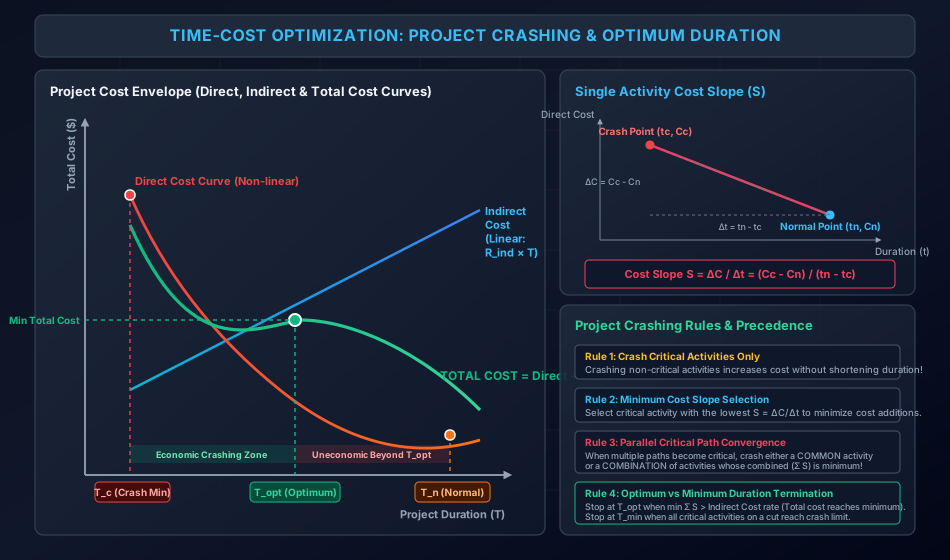
Project Crashing is the systematic, algorithmic procedure for compressing activity durations along the critical path at the lowest incremental cost. However, crashing direct activities consumes additional labor overtime, specialized equipment, and premium material deliveries, escalating Direct Costs. Concurrently, shortening project duration curtails field overheads, site administrative salaries, equipment rentals, and utility charges, reducing Indirect Costs. The interplay between these opposing economic forces creates a convex Total Cost Curve, defining an Optimum Project Duration () at which total expenditure is minimized.
Beyond temporal compression, real-world construction projects operate under finite material, labor, and plant availability. Resource Allocation resolves resource scheduling conflicts via two distinct operational philosophies:
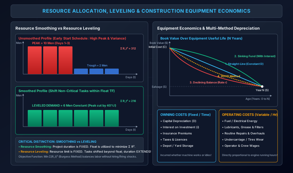
- Resource Smoothing: Retaining a fixed project completion date while shifting non-critical activities within their float boundaries to minimize resource demand fluctuations ().
- Resource Leveling: Imposing a strict ceiling on peak resource availability, inevitably extending project duration when demands exceed site capacities.
Finally, because heavy earthmoving, compaction, and hoisting machinery represent the single largest capital investment in civil construction, this module formalizes Equipment Economics: categorizing Owning Costs (capital depreciation, investment interest, insurance, taxes, depot storage) versus Operating Costs (fuel, lubricants, routine repairs, tires/tracks, operator wages), and evaluating capital depreciation across four analytical models: Straight-Line, Sinking Fund, Declining Balance, and Sum-of-the-Years'-Digits (SOYD).
2. Learning Objectives & Exam Weightage Analysis
Learning Objectives
- Define and differentiate the components of project expenditure: Direct Costs, Indirect Costs, Penalty / Liquidated Damages, and Incentive / Bonus Curves.
- Define the Normal Point , Crash Point , and derive the Activity Cost Slope equation: .
- Execute the rigorous step-by-step Project Crashing Algorithm: identifying critical paths, crashing activities with minimum cost slope, and managing parallel critical path convergence.
- Distinguish between the Optimum Project Duration () (minimum total cost) and the Minimum Physical Project Duration () (all critical paths crashed to their absolute limit).
- Plot and interpret Resource Loading Profiles, Cumulative Usage Curves, and differentiate Resource Smoothing (fixed duration, utilizes float) from Resource Leveling (fixed resource cap, extends project duration).
- Formulate the mathematical objective function for Resource Smoothing via Burgess' Minimum Sum of Squares criterion ().
- Deconstruct heavy construction equipment hourly costs into Owning Costs (fixed time-based) and Operating Costs (variable runtime-based).
- Compute annual and hourly depreciation across four classical methods: Straight-Line, Sinking Fund, Declining Balance (constant percentage), and Sum-of-the-Years'-Digits (SOYD).
Exam Weightage Analysis
| Exam Stream | Typical Question Type | Average Weightage | Recurring Focus Concepts |
|---|---|---|---|
| GATE CE | Numerical Answer Type (NAT) & MCQ | 2 – 4 Marks | Formula for cost slope; multi-stage project crashing calculations; finding optimum project duration and minimum total cost; identifying governing combination of crashing activities on parallel critical paths. |
| UPSC ESE (Prelims & Mains) | Objective + Multi-step Conventional | 12 – 24 Marks | Step-by-step network crashing tables; cost slope ranking; resource leveling vs smoothing definitions and sketches; SOYD, Sinking Fund, and Declining Balance depreciation derivations. |
| SSC JE / RRB JE | Direct Objective Questions | 3 – 5 Questions | Formula for Cost Slope (); Direct vs Indirect cost behavior with time; Straight-line depreciation formula; effect of crashing on indirect cost. |
| State PSC AE/JE | Mixed Objective & Short Problem | 4 – 8 Marks | Calculating activity cost slope; finding optimum crashing sequence; definition of salvage value; book value computation after years. |
3. Project Cost Dynamics: Direct, Indirect, Outage & Total Cost Curves
A construction project's total cost () is the superposition of multiple cost components that exhibit opposing behaviors as project duration () varies.
+---------------------------------------------------------------------------------------------------+
| COST COMPONENT      | PHYSICAL CONSTITUTION                                 | VARIATION WITH TIME |
+---------------------+-------------------------------------------------------+---------------------+
| Direct Cost (C_dir) | Direct labor, materials, equipment fuel, subcontracts | Increases as T cuts |
| Indirect Cost (C_ind| Site supervision, camp overheads, plant rent, admin   | Decreases as T cuts |
| Liquidated Damages  | Contractual delay penalties imposed beyond deadline   | Step / Linear Surge |
| Early Bonus         | Client incentive payout for ahead-of-time handover    | Step / Linear Drop  |
+---------------------+-------------------------------------------------------+---------------------+
3.1 Direct Costs ()
Direct costs are costs directly attributed to the execution of specific physical work packages:
- Labor wages (regular vs overtime).
- Construction materials and expedited freight fees.
- Equipment operating charges and deployment of high-capacity machinery.
Behavior: When an activity is performed at its normal, unhurried pace (), direct cost is minimized at the Normal Cost (). To accelerate the task to a shorter duration (), management must add labor shifts, pay overtime premiums, or deploy larger excavators. Due to diminishing marginal labor productivity and congestion on the job site, Direct Cost rises non-linearly (piecewise convex) as duration is compressed toward the Crash Duration ().
3.2 Indirect Costs ()
Indirect costs encompass site and headquarters overhead expenditures that cannot be allocated to a single activity, but accrue as a function of total elapsed project time:
- Site supervisory and engineering salaries (Project Manager, Safety Engineer, Surveyors).
- Site office rental, utilities, sanitation, security, and camp maintenance.
- Scaffolding, crane, and temporary works recurring hire charges.
- Financing interest, bank guarantee charges, and commercial insurance premiums.
Behavior: Indirect costs are directly proportional to total project duration ():
where is the daily or weekly indirect cost rate ( or ). Shortening project duration directly saves indirect costs.
3.3 Total Cost Curve ()
The Total Project Cost () at any duration is the algebraic sum of total direct and indirect costs:
As duration is compressed starting from the Normal Project Duration ():
- Initially, the daily savings in indirect cost () exceed the incremental direct crash cost (). Consequently, Total Cost decreases.
- Total Cost reaches a global minimum at the Optimum Project Duration () where the incremental direct cost slope equals the indirect cost rate:
- Compressing duration beyond requires crashing activities with steep cost slopes that exceed , causing Total Cost to increase sharply.
- Durations shorter than the Minimum Project Duration () are physically impossible because all critical activities have reached their technological crash limits ().
4. Activity Crashing Mechanics: Normal Point, Crash Point & Cost Slope
For any individual activity , two boundary operational states are defined:
        Direct Cost
            ^
            |          Crash Point (tc, Cc)
         Cc +------------*
            |           / |
            |          /  |  Cost Slope (S)
            |         /   |  S = (Cc - Cn) / (tn - tc)
            |        /    |
         Cn +-------*-----+-------------------------> Duration (t)
                    |     |
                   tc    tn
                 (Crash) (Normal)
                    <----->
                      Δt (Crash Limit)
4.1 Boundary Points
- Normal Point : The standard duration and corresponding minimum direct cost achievable under normal working hours, standard crew sizes, and conventional equipment.
- Crash Point : The minimum technologically feasible duration and its corresponding maximum direct cost achievable by utilizing maximum overtime, multi-shift 24/7 working, and redundant equipment.
4.2 Linear Cost Slope Assumption
Although real-world crashing curves can be non-linear, standard civil engineering practice assumes a linear relationship between duration and direct cost within the interval .
The Cost Slope () is the marginal direct cost incurred per unit reduction in activity duration:
where:
- Total additional direct cost required to fully crash the activity.
- Maximum allowable crash limit (crashable duration).
- Cost slope (, ).
[!IMPORTANT] The Cost Slope represents the economic "penalty" of compressing time. An activity with a low cost slope provides inexpensive schedule compression, whereas an activity with a high cost slope is expensive to accelerate.
5. Systematic Project Crashing Algorithm & Parallel Path Emergence
Project crashing must follow a rigorous, deterministic sequence to ensure the project duration is shortened at minimal incremental cost:
5.1 The Step-by-Step Crashing Procedure
+---------------------------------------------------------------------------------------------------+
| STEP 1: Compute All Normal Times & Cost Slopes                                                    |
|         Calculate S = (Cc - Cn) / (tn - tc) and maximum crash limit Δt = tn - tc for all tasks.   |
+---------------------------------------------------------------------------------------------------+
| STEP 2: Network Forward/Backward Pass                                                             |
|         Identify the project duration (T) and determine ALL network paths and the Critical Path.  |
+---------------------------------------------------------------------------------------------------+
| STEP 3: Identify Candidate Critical Activities                                                    |
|         Filter only activities lying on the CRITICAL PATH that have remaining crash capacity.     |
+---------------------------------------------------------------------------------------------------+
| STEP 4: Select Minimum Cost Slope Activity                                                        |
|         Select the critical activity with the lowest cost slope: S_min = min(S_crit).             |
+---------------------------------------------------------------------------------------------------+
| STEP 5: Determine Allowable Crash Increment (Δt_crash)                                            |
|         Δt_crash = min[ Remaining crash limit of selected activity,                              |
|                         Total Float of the nearest sub-critical path ]                            |
+---------------------------------------------------------------------------------------------------+
| STEP 6: Execute Crashing & Update Network                                                         |
|         Reduce duration by Δt_crash. Add Δt_crash * S_min to Direct Cost.                         |
|         Subtract Δt_crash * R_ind from Indirect Cost. Compute new Total Cost.                     |
+---------------------------------------------------------------------------------------------------+
| STEP 7: Check for Parallel Critical Path Emergence                                                |
|         If a sub-critical path loses all float, it becomes a NEW PARALLEL CRITICAL PATH!          |
|         To crash further, every critical path MUST be simultaneously shortened by the same Δt:   |
|           • Option A: Crash an activity COMMON to all critical paths.                             |
|           • Option B: Crash a combination of individual activities (one per path) such that       |
|                       the combined slope Σ S is minimized.                                        |
+---------------------------------------------------------------------------------------------------+
| STEP 8: Termination Criteria                                                                      |
|         • To find T_opt: Stop when minimum combined slope (min Σ S) EXCEEDS R_ind.                |
|         • To find T_min: Stop when all activities along any cut of the critical paths hit tc.     |
+---------------------------------------------------------------------------------------------------+
6. Optimum Project Duration () vs Minimum Physical Duration ()
It is crucial to differentiate between two fundamental milestones in time-cost trade-off analysis:
+---------------------------------------------------------------------------------------------------+
| PARAMETER           | OPTIMUM PROJECT DURATION (T_opt)         | MINIMUM PROJECT DURATION (T_min)         |
+---------------------+------------------------------------------+------------------------------------------+
| Definition          | Duration where TOTAL project cost is     | Shortest physically possible duration    |
|                     | minimized (Direct + Indirect = MIN).     | achievable by fully crashing all paths.  |
| Governing Rule      | Crash as long as Cost Slope S <= R_ind.  | Crash until crash capacity is exhausted. |
| Economic Feasibility| Maximum economic profit for contractor.  | Uneconomic (Total cost rises above min). |
| Total Cost State    | Global minimum of the U-curve.           | Higher than minimum, but achieves max    |
|                     |                                          | physical schedule compression.           |
+---------------------+------------------------------------------+------------------------------------------+
7. Resource Management: Loading, Profiles & Demand Histograms
In CPM network scheduling, time calculations assume that resources (labor, excavators, transit mixers, steel fixers) are available in unlimited quantities. In real-world construction, resource limits govern execution.
7.1 Resource Loading Profile & Histogram
A Resource Histogram is a bar chart displaying the total quantity of a specific resource required per day across the project duration.
- It is generated by summing the daily resource requirements of all concurrently active tasks.
- If all activities begin at their Early Start (), the early start histogram typically exhibits severe resource spikes early in the project followed by sharp troughs.
- Fluctuating resource profiles cause severe inefficiencies: excessive hiring and firing, labor demotivation, equipment idle charges, and congested site logistics.
8. Resource Smoothing vs Resource Leveling
8.1 Rigorous Comparison of Methodologies
+---------------------------------------------------------------------------------------------------+
| CHARACTERISTIC      | RESOURCE SMOOTHING                               | RESOURCE LEVELING                        |
+---------------------+------------------------------------------+------------------------------------------+
| Project Duration    | STRICTLY FIXED (Cannot be extended)      | VARIABLE (Extended beyond normal date)   |
| Critical Path       | Unaltered (Critical activities fixed)    | Extended / Altered as tasks are queued   |
| Resource Limit      | No rigid cap; goal is to balance demand  | STRICT RESOURCE CEILING (Imposed cap)    |
| Activity Movement   | Non-critical tasks shifted WITHIN FLOAT  | Tasks delayed beyond float if needed     |
| Objective Function  | Minimize demand variance: min Σ (R_t)^2  | Keep daily demand <= Resource Ceiling    |
| Practical Use       | Smoothing labor peaks to avoid layoffs   | Limited fleet (e.g., only 2 cranes site) |
+---------------------+------------------------------------------+------------------------------------------+
8.2 Burgess' Minimum Sum of Squares Criterion
For Resource Smoothing, the objective is to make the daily resource consumption as uniform as possible. The mathematically optimal schedule is that which minimizes the Sum of Squares of Daily Resource Demands:
where is the total resource quantity required on day .
- Squaring penalizes high resource peaks heavily (e.g., , whereas ).
- Shifting a task from a peak period to a trough period substantially lowers , creating a leveled, sustainable workforce demand without extending project duration.
9. Construction Equipment Fleet Economics: Owning vs Operating Costs
Heavy equipment represents over of direct costs on highway, dam, and foundation contracts. Machinery expenditures are bifurcated into two mutually exclusive financial domains:
+---------------------------------------------------------------------------------------------------+
| COST CATEGORY       | OWNING COSTS (Fixed / Capital)           | OPERATING COSTS (Variable / Runtime)     |
+---------------------+------------------------------------------+------------------------------------------+
| Nature of Cost      | Incurred purely with the PASSAGE OF TIME | Incurred ONLY when the machine is        |
|                     | (whether machine works or sits idle).    | physically running and burning fuel.     |
| Cost Components     | • Capital Depreciation (D)               | • Fuel / Electric Energy                 |
|                     | • Interest on Investment Capital (i)     | • Lubricants, Grease, Filters            |
|                     | • Commercial Insurance Premiums          | • Routine Maintenance & Wear Parts       |
|                     | • Equipment Taxes & Registration Fees    | • Undercarriage / Tires Wear             |
|                     | • Central Storage Depot / Yard Charges   | • Operator Wages & Crew Overheads        |
| Cost Metric         | Expressed per year or per owning hour    | Expressed per operating hour ($/hr)      |
+---------------------+------------------------------------------+------------------------------------------+
9.1 Average Annual Investment () for Interest, Insurance & Taxes (IIT)
Because a machine depreciates over its useful life of years from purchase price to salvage value , interest, insurance, and taxes (IIT) are charged on the Average Annual Investment ():
If salvage value :
The combined annual IIT cost is then:
10. Equipment Depreciation Methodologies & Economic Life
Depreciation is the structural loss in the monetary value of a machine over time caused by physical wear and tear, age, deterioration, and technological obsolescence.
Let:
- Initial purchase capital cost (delivered cost including freight and commissioning).
- Estimated salvage value (scrap value) at the end of useful life.
- Useful economic life in years.
- Current age of equipment in years ().
- Book Value of the equipment at the end of year .
10.1 Straight-Line Depreciation Method
The simplest and most widely used method. It assumes depreciation occurs at a constant, uniform rate throughout the asset's lifespan:
The Book Value at the end of year is:
10.2 Sinking Fund Depreciation Method
This method assumes that a uniform annual sinking fund payment () is deposited into a compound interest-bearing fund at annual interest rate . The accumulated sum at year exactly equals the total depreciable value :
The depreciation in any specific year is the annual deposit plus interest earned on previous accumulations:
The Book Value at the end of year is:
Characteristic: Depreciation is lowest in year 1 and increases geometrically in later years. The book value curve is convex upward.
10.3 Declining Balance (Constant Percentage) Method
Also known as the Reducing Balance or Matheson Method. It assumes the asset depreciates by a constant percentage rate () applied to the book value at the beginning of each year:
The depreciation in year is:
The Book Value at the end of year is:
[!NOTE] The Declining Balance method cannot be used if salvage value , as becomes (100% depreciation in Year 1). A nominal salvage value (e.g., ) is always assigned.
10.4 Sum-of-the-Years'-Digits (SOYD) Method
An accelerated depreciation method that provides high tax shields in early machine years. The digits representing the years of life are summed:
The depreciation in year is proportional to the remaining life at the start of that year :
The cumulative depreciation through year is:
The Book Value at the end of year is:
11. Step-by-Step Rigorous Worked Numerical Examples
Problem 1: Full Multi-Path Project Crashing, Parallel Path Emergence & Cost Optimization
Problem Statement:
A project network consists of 4 nodes and 4 activities:
- Path 1: Activity
- Path 2: Activity
The normal and crash parameters for each activity are:
| Activity | Normal Time (days) | Crash Time (days) | Normal Cost ($) | Crash Cost ($) |
|---|---|---|---|---|
The site indirect overhead cost rate is .
- Compute the Cost Slope and maximum allowable crash limit for each activity.
- Determine the initial Critical Path, Normal Duration (), and initial Total Project Cost.
- Perform step-by-step project crashing down to the Minimum Physical Duration ().
- Identify the Optimum Project Duration () and compute the Minimum Total Cost.
Step 1: Compute Cost Slopes () and Crash Limits ()
Using and :
- Activity :
- Activity :
- Activity :
- Activity :
Step 2: Initial Normal Schedule (Stage 0: )
- Path 1: [CRITICAL PATH]
- Path 2: [Float = 1 day]
- Normal Direct Cost
- Indirect Cost
- Initial Total Cost
Step 3: First Crashing Stage (Stage 1: Crash from 15 to 14 days)
- Critical Path: Path 1 ().
- Critical activities: [Slope , cap ] and [Slope , cap ].
- Select Activity (or ) with .
- Maximum allowable crash increment is limited by Path 2 float: .
- Crash Activity by (new , remaining cap ).
- New Project Duration: .
- Path 1 duration .
- Path 2 duration .
- Financial Impact:
- Added Direct Cost .
- Saved Indirect Cost .
- Total Cost (Net savings of ).
Step 4: Second Crashing Stage (Stage 2: Crash from 14 to 12 days)
Because both Path 1 and Path 2 are critical, to shorten the project further we must crash one activity on Path 1 AND one activity on Path 2 simultaneously:
- Available combinations:
- [Slope 200] and [Slope 200]: Combined Slope .
- [Slope 200] and [Slope 300]: Combined Slope .
- [Slope 200] and [Slope 200]: Combined Slope .
- Lowest combined slope is (via and ).
- Economic Evaluation: Further crashing will INCREASE Total Cost by !
Step 5: Continuing to Minimum Physical Duration ()
To establish the physical minimum:
-
Crash Activity by its remaining (reaches ) and Activity by (new , remaining cap ):
- Duration .
- Direct Cost .
- Indirect Cost .
-
Next increment: Activity is fully crashed. On Path 1, crash Activity [Slope 200, cap 3d]. On Path 2, crash remaining of [Slope 200]:
- Combined Slope .
- Crash by .
- Direct Cost .
- Indirect Cost .
-
Next increment: Activity is fully crashed. On Path 2, only Activity remains [Slope 300, cap 2d]. On Path 1, Activity has 2 days remaining [Slope 200]:
- Combined Slope .
- Crash by .
- Direct Cost (Notice: , perfect check!).
- Indirect Cost .
Problem 2: Resource Smoothing via Burgess' Minimum Sum of Squares Criterion
Problem Statement:
A project has a critical duration of 6 days. The network comprises three activities:
- Activity : Duration , requires (Critical: Days 1 to 3).
- Activity : Duration , requires (Critical: Days 4 to 6).
- Activity : Duration , requires (Non-critical: ).
- Determine the daily mason requirement profile and compute Burgess' sum of squares () under the Early Start Schedule ().
- Smooth the schedule by shifting non-critical activity within its float.
- Compute the new mason requirement profile, the reduction in peak demand, and the percentage reduction in .
Step 1: Early Start Schedule Analysis
Activity begins at (Days 1 to 3):
- Days 1 to 3:
- Days 4 to 6:
Mason profile:
Step 2: Resource Smoothing (Late Start Schedule)
Shift Activity by 3 days to start at Day 4 (, running on Days 4 to 6, strictly within ):
- Days 1 to 3:
- Days 4 to 6:
Smoothed mason profile:
Conclusion: Resource smoothing achieved a perfectly level workforce across all 6 days with zero extension of project duration.
Problem 3: Heavy Excavator Owning & Operating Economics & Multi-Method Depreciation
Problem Statement:
A heavy crawler hydraulic excavator ( bucket capacity) is purchased for a highway earthwork project:
- Capital Delivered Cost:
- Estimated Salvage Value: (at end of useful life)
- Useful Economic Life:
- Annual Operating Hours: (Total lifespan )
- Annual Interest, Insurance, and Taxes (IIT) rate:
- Compute the annual and hourly depreciation using:
- (a) Straight-Line Method
- (b) Sinking Fund Method (at )
- (c) Declining Balance Method
- (d) Sum-of-the-Years'-Digits (SOYD) Method for Year 1 and Year 2.
- Compute the Average Annual Investment () and the hourly owning cost (Depreciation + IIT) using Straight-Line depreciation.
- If operating expenses are: Fuel (18 L/hr @ $1.20/L), Lubricants/Filters (15% of fuel), Maintenance/Repairs (80% of straight-line depreciation), Undercarriage wear ($4.50/hr), and Operator wages ($25.00/hr), compute the total hourly equipment operating cost and the Total Hourly Owning & Operating Rate.
Step 1: Depreciation Calculations
(a) Straight-Line Method:
(b) Sinking Fund Method ():
(c) Declining Balance Method:
- Year 1 Depreciation:
- Year 2 Depreciation:
- Year 5 Check: (Exact!).
(d) Sum-of-the-Years'-Digits (SOYD) Method:
- Year 1 Depreciation: ()
- Year 2 Depreciation: ()
Step 2: Hourly Owning Cost (Straight-Line + Average Investment IIT)
Step 3: Hourly Operating Cost & Total Rate
- Fuel:
- Lubricants & Filters:
- Routine Maintenance & Repairs:
- Undercarriage Wear:
- Operator Wages & Overheads:
12. Comprehensive Exam Question Bank
Section A: GATE CE Previous Years & Anticipated Styles
-
[GATE CE NAT] The normal duration and normal cost of an activity are 10 days and $5,000, respectively. The crash duration and crash cost are 6 days and $7,400, respectively. The cost slope (in $/day) of the activity is:
- (A) 400
- (B) 600
- (C) 1200
- (D) 2400
Answer: (B) .
-
[GATE CE MCQ] While crashing a project network, which of the following rules is INCORRECT?
- (A) Crashing is done only along the critical path.
- (B) If multiple paths are critical, duration must be reduced simultaneously on all critical paths.
- (C) Crashing an activity always reduces both direct cost and indirect cost.
- (D) The process terminates when minimum cost slope exceeds the indirect cost rate for finding optimum duration.
Answer: (C). Crashing increases direct cost and decreases indirect cost.
Section B: UPSC ESE Conventional Practice
- [ESE Mains] (a) Distinguish clearly between Resource Smoothing and Resource Leveling with neat sketches. State the objective function of Burgess' method.
(b) An earthmoving machine costing Rs. 25,00,000 has an estimated life of 6 years and scrap value of Rs. 2,50,000. Determine the book value of the machine at the end of 4 years using the Sum-of-the-Years'-Digits (SOYD) method.
Solution Outline for (b): . .
Cum depreciation for 4 years .
Book Value .
Section C: SSC JE & State AE/JE Quick Fire
-
The cost slope is given by the formula:
- (A)
- (B)
- (C)
- (D)
Answer: (A) .
-
In resource smoothing, which parameter remains strictly CONSTANT?
- (A) Total project duration
- (B) Daily labor demand
- (C) Daily equipment hours
- (D) Independent float of all tasks
Answer: (A) Total project duration.
-
Under the Straight-Line method of depreciation, annual depreciation is:
- (A) Increasing with time
- (B) Decreasing with time
- (C) Constant throughout life
- (D) Zero in the first year
Answer: (C) Constant throughout life ().
-
In the Declining Balance method, the depreciation rate cannot be calculated if:
- (A) years
- (B) Salvage value
- (C)
- (D) Interest rate is zero
Answer: (B) Salvage value ( requires ).
13. Common Conceptual Pitfalls & Field Traps
- The Cost Slope Denominator Order Trap:
Writing in the denominator instead of . Because and , both numerator and denominator must be positive: . - Crashing Non-Critical Activities:
Selecting an activity with the lowest cost slope in the entire network even though it is non-critical. Crashing a non-critical activity burns money without shortening the project by even one hour! - The Parallel Path Uncoordinated Crash Trap:
When two paths become critical, crashing only one of them. Both paths must be crashed simultaneously; otherwise, the un-crashed critical path continues to govern project duration and the crash expenditure is completely wasted. - Confusing Leveling with Smoothing:
Assuming resource leveling maintains project duration. Leveling imposes a hard cap and almost always delays project delivery. Smoothing preserves the contractual finish milestone. - Zero Salvage Fallacy in Constant Percentage Depreciation:
Attempting to use Declining Balance with . In textbook problems where salvage value is unstated for declining balance, assume a standard salvage value.
14. Quick Reference Formulas & Multi-Code Summary Table
| Category | Parameter | Exact Analytical Formulation |
|---|---|---|
| Crashing Metrics | Activity Cost Slope () | |
| Crash Limit () | ||
| Total Project Cost () | ||
| Optimum Duration Condition | ||
| Resource Smoothing | Burgess Objective Function | (Duration fixed) |
| Equipment Capital | Average Annual Investment () | |
| Depreciation Models | Straight-Line Depreciation () | |
| Sinking Fund Annual Deposit () | ||
| Declining Balance Rate () | ||
| Declining Balance Book Value | ||
| SOYD Year Depreciation () | ||
| Equipment Rates | Total Hourly Equipment Rate |