Project Planning, Work Breakdown Structure (WBS), Bar Charts, Milestone Charts & Network Logic
In this chapter (1 topics)
On this page
- 1. Module Overview & Pedagogical Scope
- 2. Learning Objectives & Exam Weightage Analysis
- Learning Objectives
- Exam Weightage Analysis
- 3. Project Management Fundamentals & The 4 Ms of Construction
- 3.1 The 4 Ms of Construction
- 3.2 The Project Life-Cycle Phases
- 4. Work Breakdown Structure (WBS) & Scope Decomposition
- 4.1 The Hierarchy Levels of WBS
- 4.2 The 100% Rule of WBS
- 5. Bar Charts (Gantt Schedules) & Milestone Charts: Architecture & Critical Flaws
- 5.1 Architecture of Henry Gantt's Bar Chart (1917)
- 5.2 Merits of Bar Charts
- 5.3 Inherent Limitations & Fatal Flaws of Bar Charts
- 5.4 Milestone Charts
- 6. Resource Aggregation Histograms & Cumulative Cash S-Curves
- 6.1 Resource Aggregation (Histogram)
- 6.2 The Cumulative Cash Flow S-Curve
- 6.3 The Project "Banana Curve" Cash Envelope
- 7. Network Fundamentals: Events, Activities & Topological Logic
- 7.1 Elements of an AOA (Activity-on-Arrow) Network
- 8. Dummy Activities: Grammatical vs Logical Dummies
- 8.1 Grammatical Dummy
- 8.2 Logical Dummy
- 8.3 Redundant Dummy
- 9. Network Integrity: Cycling, Dangling & Validation Rules
- 10. Fulkerson's Numbering Algorithm & AON Precedence Diagramming (PDM)
- 10.1 Fulkerson's Event Numbering Algorithm
- 10.2 Activity-on-Node (AON) / Precedence Diagramming Method (PDM)
- 11. Step-by-Step Rigorous Worked Numerical Examples
- Problem 1: AOA Network Construction, Dummy Identification & Fulkerson Numbering
- Problem 2: Resource Histogram Aggregation & Cash S-Curve
- Problem 3: AON Precedence Logic with Leads and Lags
- 12. Comprehensive Exam Question Bank
- Section A: GATE CE Previous Years & Anticipated Styles
- Section B: UPSC ESE Conventional Practice
- Section C: SSC JE & State AE/JE Quick Fire
- 13. Common Conceptual Pitfalls & Field Traps
- 14. Quick Reference Formulas & Multi-Code Summary Table
1. Module Overview & Pedagogical Scope
Modern civil engineering projects—high-speed rail corridors, multi-span bridges, super-tall towers, hydroelectric dams, and multi-lane expressways—are large-scale, complex socio-technical systems characterized by massive capital investments, tight deadlines, interdisciplinary technical teams, and severe environmental constraints. Delivering these capital assets within budgeted costs and targeted timelines demands structured, quantitative project planning and control techniques.
Historically, project scheduling relied upon visual representations such as the Gantt Bar Chart (developed by Henry Gantt during World War I). While bar charts provide intuitive visual communication on construction jobsites, their inability to depict activity interdependencies, identify critical bottlenecks, or accommodate uncertainty led to the development of mathematical graph-theoretic network techniques: the Critical Path Method (CPM) and the Program Evaluation and Review Technique (PERT).
This introductory master module for Subject 13 establishes:
- Construction Management Principles: Management frameworks, project life-cycle phases, and the orchestration of the "4 Ms" of construction: Men (Labor), Materials, Machinery (Equipment), and Money (Capital).
- Work Breakdown Structure (WBS): Systematic hierarchical scope decomposition from the complete project down to sub-projects, work packages, and discrete measurable activities following the rule.
- Bar Charts & Milestone Charts: Graphical mechanics, operational advantages on the jobsite, and four fatal mathematical limitations.
- Resource Aggregation & Cash S-Curves: Daily/weekly labor and cost histograms, peak demand detection, and cumulative sigmoidal expenditure curves (the Project Cash S-Curve and the Early/Late Start "Banana Curve" envelope).
- Network Topology & Logic: Directed acyclic graphs, Activity-on-Arrow (AOA) mechanics, tail and head events, concurrent/preceding/succeeding activities, and dummy activities (grammatical vs logical).
- Network Integrity & Numbering: Detection and elimination of looping/cycling, dangling, and redundancy errors, Fulkerson's Event Numbering Algorithm (), and Activity-on-Node (AON) / Precedence Diagramming Method (PDM) dependency relationships.
2. Learning Objectives & Exam Weightage Analysis
Learning Objectives
- Explain the project life-cycle phases and construct a multi-level Work Breakdown Structure (WBS) down to work package level.
- Construct and critique Gantt bar charts, milestone charts, and resource aggregation histograms, and derive the cumulative S-curve.
- Differentiate between grammatical dummies and logical dummies in Activity-on-Arrow (AOA) networks and eliminate redundant dummies.
- Detect topological network errors (cycling/looping, dangling events, duplicate activity identifiers) in complex network configurations.
- Apply Fulkerson's rule to number all network events systematically such that the tail event index is strictly less than the head event index for every directed arrow.
- Formulate Activity-on-Node (AON) / Precedence Diagramming Method (PDM) relationships: Finish-to-Start (), Start-to-Start (), Finish-to-Finish (), and Start-to-Finish () with leads and lags.
Exam Weightage Analysis
| Exam Stream | Typical Question Type | Average Weightage | Recurring Focus Concepts |
|---|---|---|---|
| GATE CE | Conceptual Multiple Choice (MCQ) & NAT | 1 – 2 Marks | Dummy activity identification, minimum dummies in network, Fulkerson rule condition (), AON lead/lag calculations. |
| UPSC ESE (Prelims & Mains) | Objective + Multi-step Conventional | 10 – 18 Marks | Limitations of bar charts, construction of AOA network with minimum dummies, resource leveling vs smoothing, WBS 100% rule. |
| SSC JE / RRB JE | Objective (Conceptual & Definitions) | 2 – 4 Questions | Definition of dummy activity (zero time/cost), Fulkerson rule, inventor of bar chart (Henry Gantt), milestone chart features. |
| State PSC AE/JE | Mixed Objective & Short Problem | 3 – 6 Marks | Minimum dummies required for given precedence tables, looping error identification, Cash S-curve characteristics. |
3. Project Management Fundamentals & The 4 Ms of Construction
Construction project management is the art and science of coordinating human, financial, physical, and technological resources throughout a project's life cycle to achieve predetermined objectives of scope, quality, time, and cost.
3.1 The 4 Ms of Construction
- Men (Labor): Skilled, semi-skilled, and unskilled workforce. Labor productivity is the most volatile variable on a construction site, susceptible to weather, motivation, supervision, and site logistics.
- Materials: Consumable physical inputs (cement, structural steel, aggregate, timber, admixtures, pipes, cables). Materials constitute of the direct capital cost of civil construction.
- Machinery (Equipment): Heavy construction plants (earthmovers, tower cranes, transit mixers, concrete pumps, asphalt batching plants, piling rigs). Involves high capital investment and ownership versus operating economics.
- Money (Finance): Capital cash flow, working capital, progress billing, retention money, bank guarantees, and contingency reserves.
3.2 The Project Life-Cycle Phases
- Concept & Feasibility Phase: Identifying the infrastructure need, conducting pre-feasibility and detailed project reports (DPR), financial viability analysis (Internal Rate of Return IRR, Cost-Benefit Ratio CBR), and Environmental Impact Assessment (EIA).
- Engineering & Detailed Design Phase: Architectural drafting, structural design (IS 456, IS 800), geotechnical soil investigation, bill of quantities (BOQ), and preparation of tender documents.
- Tendering & Procurement Phase: Notice Inviting Tender (NIT), pre-qualification, bid evaluation, award of contract, and signing of legal agreement.
- Construction Execution Phase: Site mobilization, layout surveying, structural erection, quality control tests, site safety audits, progress monitoring against baseline schedules.
- Commissioning & Handover Phase: Non-destructive testing, load testing of bridges, system dry runs, snag list clearance, as-built drawing preparation, and formal transfer of physical possession to the owner/client.
- Operations & Maintenance (O&M): Defect Liability Period (DLP), routine maintenance, and asset management.
4. Work Breakdown Structure (WBS) & Scope Decomposition
A Work Breakdown Structure (WBS) is a deliverables-oriented hierarchical decomposition of the total scope of work to be carried out by the project team.
4.1 The Hierarchy Levels of WBS
Level 1: Total Project (e.g., Elevated Metro Rail Line 1 - 25 km)
   │
   ├── Level 2: Sub-Projects / Major Packages (e.g., Viaduct Civil, Stations, Trackwork, Traction)
   │      │
   │      ├── Level 3: Sub-Networks / Components (e.g., Station Pier Foundations, Pier Caps, Girders)
   │      │      │
   │      │      ├── Level 4: Work Packages (e.g., Pier Piling Group 14 to 28)
   │      │      │      │
   │      │      │      └── Level 5: Discrete Activities (e.g., Rig setup, Bore boring, Cage lowering, Concreting)
4.2 The 100% Rule of WBS
The Rule states that the WBS must capture of the work defined by the project scope, including internal project management, QA/QC, and safety.
- The sum of work at each "child" level must equal of the work represented by the "parent" element.
- No work outside the scope should be included, and no work within the scope should be omitted.
- Work Package: The lowest level of the WBS where cost and duration can be reliably estimated, scheduled, monitored, and assigned to a single responsible organizational unit (Cost Account).
5. Bar Charts (Gantt Schedules) & Milestone Charts: Architecture & Critical Flaws
5.1 Architecture of Henry Gantt's Bar Chart (1917)
A bar chart consists of two orthogonal coordinate axes:
- Vertical Axis: A sequential list of all construction activities.
- Horizontal Axis: A linear calendar time scale (hours, days, weeks, months).
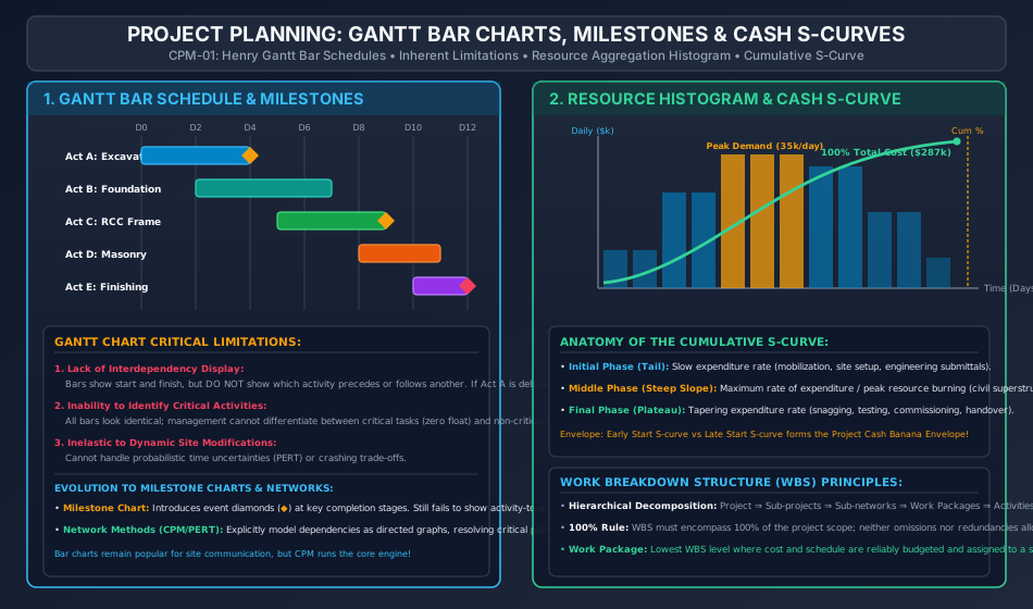
- Each activity is plotted as a horizontal bar whose left end marks the scheduled start, whose length represents the planned duration (), and whose right end marks the scheduled completion date.
5.2 Merits of Bar Charts
- Highly intuitive visual appeal; easily comprehended by non-technical stakeholders, tradesmen, and site foremen.
- Excellent for displaying overall project duration and broad progress milestones.
- Readily displays physical percentage completion by hatching/shading the active bars.
5.3 Inherent Limitations & Fatal Flaws of Bar Charts
Despite their widespread visual usage, bar charts suffer from four critical deficiencies:
- Lack of Activity Interdependency (Precedence Logic):
Bars do not show which task must finish before another can begin. If Activity is delayed by 4 days, the bar chart fails to indicate whether Activity can proceed independently or must stall, hiding the ripple effect. - Inability to Identify the Critical Path:
All bars appear visually identical. Management cannot distinguish between critical activities (whose delay delays the entire project) and non-critical activities (which possess buffer time or float). - No Representation of Uncertainties:
Bar charts are strictly deterministic. They assume static, fixed task durations and cannot model probabilistic variations or stochastic weather impacts (as handled by PERT). - Cumbersome Progress Updating:
Dynamic site modifications cannot be recalculated automatically. Updating a delayed bar chart requires redrawing the entire schedule manually.
5.4 Milestone Charts
To mitigate the lack of dependencies in pure bar charts, Milestone Charts were introduced. Key project events of special importance—such as "Foundation Concrete Completed", "Boiler Drum Lifted", or "Substation Energized"—are marked as distinct geometric symbols (typically diamonds or circles ) on the bar chart.
- Limitation: While milestones highlight critical dates, they still fail to show activity-to-activity logic and cannot compute mathematical floats.
6. Resource Aggregation Histograms & Cumulative Cash S-Curves
6.1 Resource Aggregation (Histogram)
By projecting the daily resource consumption (manpower, equipment hours, daily expenditure) of each active bar down onto the horizontal time axis and summing them vertically, a Resource Aggregation Histogram is obtained.
- Highlights peak resource demands (e.g., maximum daily skilled masons or maximum daily concrete transit mixer trucks).
- In unconstrained scheduling, resource histograms display erratic spikes and valleys, leading to inefficient hiring/firing of labor and idle equipment costs.
- Serves as the raw baseline for Resource Leveling (smoothing peaks within float limits) and Resource Allocation (shifting activities under hard resource ceilings).
6.2 The Cumulative Cash Flow S-Curve
When the cumulative expenditure of a project is plotted as a function of time, it universally assumes a characteristic sigmoidal "S" shape:
- Initial Tail (Slow Ramp-Up): Early project stage characterized by low expenditure rates during mobilization, topographical surveying, geotechnical testing, submittals, and permits.
- Central Stem (Steep Maximum Slope): Middle execution stage where primary civil, structural, and electro-mechanical work proceeds simultaneously. Peak daily cash burn rate ().
- Upper Plateau (Tapering Off): Final closing stage characterized by diminishing expenditure during architectural snagging, testing, dry runs, commissioning, and handover.
6.3 The Project "Banana Curve" Cash Envelope
If a project is scheduled with all activities starting at their Earliest Start Times (), the resulting cumulative cost curve forms the upper boundary. If all activities are scheduled at their Latest Start Times (), the resulting curve forms the lower boundary. The enclosed area between the Early-Start S-curve and Late-Start S-curve is known as the Banana Envelope:
- Any actual site progress curve falling inside the banana envelope represents a feasible, controlled project.
- Crossing below the Late-Start curve indicates an irreversible project delay that directly postpones final project completion!
7. Network Fundamentals: Events, Activities & Topological Logic
A network is a directed acyclic graph (DAG) representing the operational sequence and interdependencies of all activities comprising a project.
7.1 Elements of an AOA (Activity-on-Arrow) Network
- Activity: A distinct, identifiable task or operation that consumes time and resources (men, material, equipment, money).
- Represented by a directed straight arrow ().
- Length, orientation, and slope of the arrow have no mathematical significance.
- Identified by its boundary nodes , where is the tail event and is the head event.
- Event (Node): An instantaneous accomplishment or milestone representing the beginning or completion of an activity.
- Represented by a geometric node (circle , square, or rectangle).
- An event consumes zero time and zero resources.
- Tail Event (): Event marking the start of an activity.
- Head Event (): Event marking the finish of an activity.
- Burst Event: A single event from which multiple activities diverge.
- Merge Event: A single event into which multiple activities converge.
8. Dummy Activities: Grammatical vs Logical Dummies
A Dummy Activity is a simulated, artificial arrow introduced into an AOA network solely to maintain structural logic.
Dummies are represented graphically by a dashed line arrow ().
8.1 Grammatical Dummy
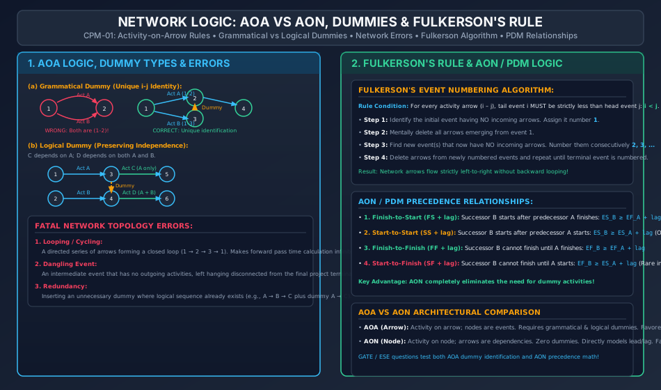
In computerized scheduling software, every activity must be uniquely identified by its tail and head node numbers .
- If two or more concurrent activities (e.g., and ) start from the same initial node and terminate at the same completion node , both would be designated as . This creates ambiguity.
- Remedy: A new intermediate event is inserted, and a grammatical dummy is added (e.g., Activity becomes , Activity becomes , and dummy connects ).
8.2 Logical Dummy
Used to enforce true sequential predecessor relationships without creating false, unintended dependencies.
- Scenario: Activity depends strictly on Activity . Activity depends on both Activity and Activity .
- Incorrect Layout: If both and terminate at node , and both and originate from node , then Activity would falsely become dependent on Activity !
- Correct Layout: Activity terminates at node ; Activity originates from node (depends only on ). Activity terminates at node . A dashed logical dummy arrow is drawn from node . Activity originates from node (depends on directly and on via the dummy).
8.3 Redundant Dummy
A dummy activity that repeats a dependency sequence already established by other direct or indirect paths is redundant and must be pruned to avoid computational clutter.
- If path exists, a dummy drawn directly from is redundant.
9. Network Integrity: Cycling, Dangling & Validation Rules
A valid CPM/PERT network must strictly comply with the following topological axioms:
- No Looping (Cycling Error):
Arrows must flow continuously forward in time. No sequence of activities can form a closed loop returning to an earlier event (). Looping creates infinite time accumulation during forward pass calculations. - No Dangling Events:
No activity arrow may be left disconnected. Every event—except the initial project start node and the final terminal completion node—must have at least one incoming arrow and at least one outgoing arrow. A disconnected intermediate branch is a dangling error. - Single Start and Single Finish Rule:
A project must have exactly one initial origin event and exactly one terminal end event. If multiple parallel tasks initiate or conclude the project, they must merge into single boundary nodes. - Arrow Unidirectionality:
Arrows can cross each other if necessary (using an arched bridge graphic), but arrows must point strictly in the direction of time progress (generally left to right).
10. Fulkerson's Numbering Algorithm & AON Precedence Diagramming (PDM)
10.1 Fulkerson's Event Numbering Algorithm
Developed by D. R. Fulkerson in 1962, this algorithm provides a systematic procedure for numbering all events in an AOA network such that for every directed arrow :
(The tail node index is strictly smaller than the head node index, eliminating backward looping).
The 4-Step Fulkerson Procedure:
- Step 1: Locate the initial event of the project (an event having only outgoing arrows and zero incoming arrows). Assign it number .
- Step 2: Mentally delete or cross out all arrows originating from event . This exposes one or more new events that now have zero incoming arrows.
- Step 3: Number these newly uncovered events consecutively as in any arbitrary order.
- Step 4: Mentally delete all arrows emerging from the newly numbered events. Repeat the process until the final terminal event is assigned the highest integer index .
10.2 Activity-on-Node (AON) / Precedence Diagramming Method (PDM)
In modern construction scheduling software (such as Primavera P6 and Microsoft Project), the Activity-on-Node (AON) method has largely superseded AOA:
- Activities are represented by nodes (rectangles or circles).
- Arrows represent dependency constraints (finish-to-start, start-to-start, etc.).
- Zero Dummies: Dummy activities are completely eliminated!
The Four PDM Dependency Relationships:
- Finish-to-Start ():
Successor activity cannot begin until predecessor finishes, plus any specified buffer lag time: (The standard relationship in traditional CPM/PERT; if lag , ). - Start-to-Start ():
Successor activity cannot start until predecessor has started and progressed by a specified lead/lag: (Used for fast-tracking pipelined civil works, e.g., structural backfilling starts 3 days after pipe laying commences). - Finish-to-Finish ():
Successor activity cannot finish until predecessor finishes, plus a lag: - Start-to-Finish ():
Successor activity cannot finish until predecessor starts: (Rarely utilized in civil engineering; used in shift changeover logistics).
11. Step-by-Step Rigorous Worked Numerical Examples
Problem 1: AOA Network Construction, Dummy Identification & Fulkerson Numbering
Problem Statement:
A civil engineering construction project consists of 9 distinct work activities. The precedence requirements among the activities are defined as follows:
- Activity : Predecessors = None
- Activity : Predecessors = None
- Activity : Predecessor =
- Activity : Predecessors =
- Activity : Predecessor =
- Activity : Predecessor =
- Activity : Predecessors =
- Activity : Predecessors =
- Activity : Predecessors =
- Analyze the precedence logic and determine where dummy activities are strictly necessary.
- Construct the complete Activity-on-Arrow (AOA) network with the minimum number of dummy activities.
- Apply Fulkerson's rule to number all network events systematically and verify that holds for every activity.
Step 1: Logic and Dummy Analysis
- Analysis of Initial Tasks: and have no predecessors, so both emerge from initial project start event .
- Dependency of :
- depends ONLY on .
- depends ONLY on .
- depends on BOTH and .
- Trap: If and terminate at a shared node, would falsely depend on , and would falsely depend on .
- Resolution: Let terminate at event (from which begins directly). Let terminate at event (from which begins directly).
- Create a new event where begins. Connect event with dummy , and connect event with dummy . Now depends on both and , while and remain independent!
- Dependency of :
- depends ONLY on . Let terminate at event , from which originates directly.
- terminates at event . Neither (which needs ) nor (which needs ) can originate directly at event if or were merged into event , because merging into would falsely make depend on , while merging into would falsely make depend on .
- Since has no successor other than , let terminate directly at event (the tail event of ), and introduce dummy from event . Now event has exact predecessors !
- Create event as the tail event of , and connect event with dummy and event with dummy . Now event has exact predecessors !
- Finally, merge , , and into event , from which terminal activity originates.
- Minimum Number of Dummies Required: () across events (Note: if also required an isolated head node, dummies would be needed; terminating directly at event saves dummy).
Step 2: System Event Topology & Fulkerson Numbering
Applying Fulkerson's rule:
- Event : Initial start node (predecessor to and ).
- Event : Head of , tail of and dummy .
- Event : Head of , tail of and dummy .
- Event : Merging head of dummies , tail of .
- Event : Head of , tail of and dummy .
- Event : Head of , tail of dummies and .
- Event : Merging head of dummies , tail of .
- Event : Merging head of and dummy , tail of .
- Event : Merging head of , tail of .
- Event : Terminal project completion event (head of ).
Verification of across all activities and dummies:
- [OK]
- [OK]
- [OK]
- [OK]
- [OK]
- [OK]
- [OK]
- [OK]
- [OK]
- [OK]
- [OK]
- [OK]
- [OK]
- [OK] Every single arrow points from a lower-numbered event to a higher-numbered event ().
Problem 2: Resource Histogram Aggregation & Cash S-Curve
Problem Statement:
A commercial warehouse expansion project consists of 5 overlapping activities with planned schedule days and uniform daily expenditure:
- Activity (Excavation): Days 1 to 4, Daily cost = $10,000/day
- Activity (Foundation): Days 3 to 7, Daily cost = $15,000/day
- Activity (Superstructure): Days 5 to 9, Daily cost = $20,000/day
- Activity (Masonry & Roof): Days 8 to 11, Daily cost = $12,000/day
- Activity (Services & Finishes): Days 10 to 12, Daily cost = $8,000/day
Compute:
- The daily expenditure profile for all 12 days.
- The peak daily funding demand and identify the peak days.
- The total project capital cost.
- Construct the cumulative expenditure table and verify the characteristics of the cumulative S-curve.
Step 1: Compute Daily Expenditure by Vertical Aggregation
- Day 1: Activity active
- Day 2: Activity active
- Day 3: Activities active
- Day 4: Activities active
- Day 5: Activities active
- Day 6: Activities active
- Day 7: Activities active
- Day 8: Activities active
- Day 9: Activities active
- Day 10: Activities active
- Day 11: Activities active
- Day 12: Activity active
Step 2: Peak Daily Demand
Step 3: Total Project Cost
Step 4: Cumulative Expenditure & S-Curve Values
| Day () | Active Activities | Daily Cost ($k) | Cumulative Cost ($k) | Cumulative % of Budget |
|---|---|---|---|---|
| 1 | ||||
| 2 | ||||
| 3 | ||||
| 4 | ||||
| 5 | ||||
| 6 | ||||
| 7 | ||||
| 8 | ||||
| 9 | ||||
| 10 | ||||
| 11 | ||||
| 12 |
S-Curve Check: The curve exhibits a slow initial slope (spending only in the first 2 days), a steep linear rise between Days 3 and 8 ( accumulated), and a smooth horizontal asymptote plateauing to on Day 12.
Problem 3: AON Precedence Logic with Leads and Lags
Problem Statement:
In a highway flyover project, two major structural operations are scheduled using the Precedence Diagramming Method (AON):
- Activity (Fabrication of Precast Prestressed Girders): Duration , begins at project day .
- Activity (Erection of Girders by Launcher Gantry): Duration .
The project specifications mandate two simultaneous precedence constraints between and :
- Constraint 1 (Start-to-Start): Erection cannot begin until at least 4 days of girder fabrication are completed: .
- Constraint 2 (Finish-to-Finish): Erection cannot be completed until at least 2 days after all girder fabrication is finalized: .
Determine:
- The Early Start () and Early Finish () of Activity .
- Which constraint actively governs the schedule of Activity .
- The total combined elapsed duration for completing both operations.
Step 1: Compute Times for Predecessor Activity
Step 2: Formulate Precedence Constraints for Activity
-
From Constraint 1 ():
Since , this constraint implies:
-
From Constraint 2 ():
Since , this constraint implies:
Step 3: Determine Governing Values
To satisfy both physical conditions simultaneously, the early finish of must satisfy the maximum requirement:
Step 4: Governance and Elapsed Duration
- Governing Constraint: Constraint 1 () strictly governs the start of Activity .
- Constraint 2 () is automatically satisfied with 4 days of positive buffer ().
- Total Combined Elapsed Project Duration: .
12. Comprehensive Exam Question Bank
Section A: GATE CE Previous Years & Anticipated Styles
-
[GATE CE] A dummy activity in a project network:
- (A) Consumes time but no resources
- (B) Consumes resources but no time
- (C) Consumes neither time nor resources
- (D) Consumes both time and resources
Answer: (C). A dummy is a purely mathematical construct consuming zero duration and zero resources.
-
[GATE CE] In an Activity-on-Arrow (AOA) network, Fulkerson's rule for numbering events ensures that:
- (A) All activities have equal floats
- (B) The initial event is numbered 0
- (C) For every activity arrow , the condition is satisfied
- (D) Critical path events are numbered with even numbers
Answer: (C).
Section B: UPSC ESE Conventional Practice
- [ESE Mains] State five major shortcomings of Henry Gantt's Bar Chart system for scheduling major civil infrastructure works. Explain how the milestone chart partially addresses these flaws and why the network method (CPM/PERT) is mathematically superior.
Section C: SSC JE & State AE/JE Quick Fire
- The rule of event numbering in network analysis is known as:
- (A) Newton's rule
- (B) Simpson's rule
- (C) Fulkerson's rule
- (D) Bowditch's rule
Answer: (C) Fulkerson's rule.
- In a project cumulative cost S-curve, the steepest slope of the curve represents the period of:
- (A) Project mobilization
- (B) Peak expenditure and maximum construction activity
- (C) Project commissioning and closeout
- (D) Tendering and contract award
Answer: (B).
- An intermediate event in a network that has incoming arrows but no outgoing arrows is termed:
- (A) Looping error
- (B) Dangling error
- (C) Burst event
- (D) Dummy event
Answer: (B) Dangling error.
13. Common Conceptual Pitfalls & Field Traps
- Dummy Necessity Overuse Trap:
Inserting dummy arrows between every pair of sequential tasks.
Field Reality: Dummies must be held to the absolute mathematical minimum. Over-dummying clutters the network, increases matrix sizes in software solvers, and introduces false critical paths. - Grammatical vs Logical Confusion:
Assuming all dummies serve the same purpose. Grammatical dummies exist solely to ensure unique identity in AOA; logical dummies preserve independent task relationships. - Bar Chart Progress Updating Fallacy:
Believing a Gantt chart can dynamically adjust to site delays. When a non-critical activity with float is delayed, an engineer cannot tell from a bar chart whether the project completion date is threatened without conducting a full CPM network pass. - Fulkerson Numbering Arbitrary Node Trap:
Assigning event numbers randomly as nodes are sketched. Random numbering violates , creates negative coordinate indexing in software algorithms, and obscures cyclic loops. - AON Lead/Lag Direction Trap:
Subtracting lag instead of adding it. A positive lag in delays the start of the successor, moving its start time forward on the calendar ().
14. Quick Reference Formulas & Multi-Code Summary Table
| Category | Parameter | Exact Analytical Formulation / Rule |
|---|---|---|
| Gantt Schedules | Activity Representation | Horizontal bar of length against calendar time |
| Milestone Symbol | Event diamond () marking major completion milestone | |
| Cash S-Curve | Daily Cash Demand | |
| Cumulative S-Curve | ||
| Envelope Bounds | Upper Bound = Early Start () S-curve; Lower Bound = Late Start () S-curve | |
| AOA Network Elements | Activity | Consumes time () and resources; arrow |
| Event Node | Instant of time; consumes ; circle | |
| Dummy Activity | Zero time (), zero cost; dashed arrow | |
| Network Integrity | Fulkerson's Condition | for every directed arrow |
| Network Errors | Looping (cycling ); Dangling (unconnected dead-end) | |
| AON / PDM Precedence | Finish-to-Start () | |
| Start-to-Start () | ||
| Finish-to-Finish () | ||
| Start-to-Finish () | ||
| WBS Standard | 100% Rule | Hierarchy must capture of scope; no omissions, no extras |